Entanglement is usually described in terms of a physical theory, namely quantum theory (QT), wherein the entities formally represented in the theory are physical entities, e.g., electrons, photons, composites (ensembles) of any size. In contrast, I will describe entanglement in the context of an information processing model in which the entities formally represented in the theory are items of information. Of course, any item of information, even a single bit, is ultimately physically reified somewhere, even if only in the physical brain of a theoretician imagining the item. So, we might expect the two descriptions of entanglement, one in terms of a physical theory and the other in terms of an information processing theory, to coalesce, to become equivalent, cf. Wheeler’s “It from Bit”. This essay works towards that goal.

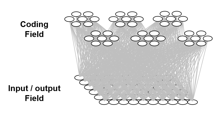
The information processing model used here is based on representing items of information as sets, specifically, (relatively) small subsets, of binary representational units chosen from a much larger universal set of these units. This type of representation has been referred to as a sparse distributed representation (SDR) or sparse distributed code (SDC).¹ We’ll use the term, SDC. Fig. 1 shows a small toy example of an SDC model. The universal set, or coding field (or memory), is organized as a set of Q=6 groups of K=7 binary units. These groups function in winner-take-all (WTA) fashion and we refer to them as competitive modules (CMs). The coding field is completely connected to an input field of binary units, organized as a 2D array (e.g., a primitive retina of binary pixels), in both directions, a forward matrix of binary connections (weights) and a reverse matrix of binary weights. All weights are initially zero. We impose the constraint that all inputs have the same number of active pixels, S=7.

The storage (learning) operation is as follows. When an input item, I_i, is presented (activated in the input field), a code, φ(I_i) consisting of Q units, one in each of the Q CMs, is chosen and activated and all forward and reverse weights between active input and active coding field units are set to one. In general, some of those weights may already be one due to prior learning. We will discuss the algorithm for choosing the codes during learning in a later section. For now, we can assume that codes are chosen at random. In general, any given coding, α, unit will be included in the codes of multiple inputs. For each new input in whose code α is included, if that input includes units (pixels) that were not active in any of the prior inputs in whose codes α was included, the weights from those pixels to α will be increased. Thus, the set of input units having a connection with weight one onto α can only increase with time (with further inputs). We call that set of input units with w=1 onto α, α’s tuning function (TF),

The retrieval operation is as follows. An input, i.e., a retrieval cue, is presented, which causes signals to travel to the coding field via the forward matrix, whereupon the coding field units compute their input summations and the unit with the max sum in each CM is chosen winner, ties broken at random. Once this “retrieved” code is activated, it sends signals via the reverse matrix, whereupon, the input units compute their input summations and are activated (or possibly deactivated) depending on whether a threshold is exceeded. In this way, partial input cues, i.e., with less than S active units, can be “filled in” and novel cues that are similar enough to previously (learned) inputs can cause the codes of such, closest-matching learned inputs to activate, which can then cause (via the reverse signals) activation of that closest-matching learned input.

With the above description of the model’s storage and retrieval operations in mind, I will now describe the analog of quantum entanglement in this classical model. Fig. 2 shows the event of storing the first item of information, I₁, into this model. I₁ consists of the S=7 light green input units. The Q=6 green coding field units are chosen randomly to be I₁‘s code, φ(I₁), and the black lines show some of the weights that would be increased, from 0 to 1, in this learning event. Each line represents both the forward and reverse weight connecting the two units. More specifically, the black lines show all the forward/reverse weights that would be increased for two of φ(I₁)’s units, denoted α and β. Note that immediately following this learning event (the storage of I₁), α and β have exactly the same TF. In fact, all six units comprising φ(I₁) have exactly the same TF. In the information processing realm, and more pointedly in neural models, we would describe these six units as being completely correlated. That is, all possible next inputs to the model, a repeat presentation of I₁ or any other possible input, would cause exactly the same input summation to occur in all six units, and thus, exactly the same response by all six units. In other words, all six units carry exactly the same information, i.e., are completely redundant.²

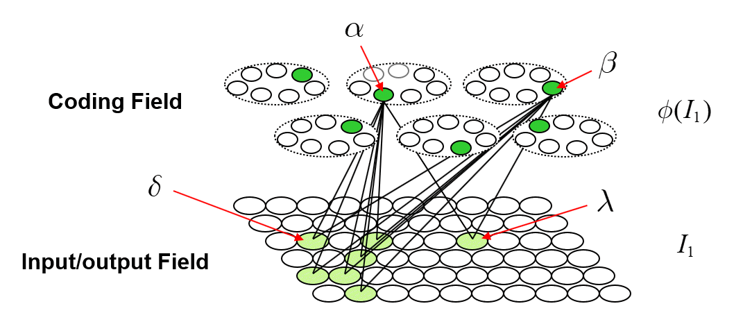
As the reader may already have anticipated, I will claim that these six units are completely entangled.³ We can consider the act of assigning the six units as the code, φ(I₁), as analogous to an event in which a particle decays, giving rise, for example, to two completely entangled photons. In the moment when the two particles are born out of the vacuum, they are completely entangled and likewise, in the moment when the code, φ(I₁), is formed, the six units comprising it are completely entangled. However, in the information processing model described here, the mechanism that explains the entanglement, i.e., the correlation, is perfectly clear: it’s the correlated increases to the forward/reverse weights to/from the six units that entangles those units. Note in particular, that there are no direct physical connections between coding field units in different CMs. This is crucial: it highlights the fact that in this explanation of entanglement, the hidden variables are external, i.e., non-local, to the units that are entangled. The hidden variables ARE the connections (weights). This hints at the possibility that the explanation of entanglement herein comports with Bell’s theorem. The 2015 results proving Bell’s theorem, explicitly rule out only local hidden variables explanations of entanglement. Fig. 3 shows the broad correspondence between the information theory and the physical theory proposed here.

Suppose we now activate just one of the seven input units comprising I₁, say δ. Then φ(I₁) will activate in its entirety (i.e., all Q=6 of its units) due to the “max sum” rule stated above, and then the remaining six input units comprising I₁ will be activated based on the inputs via the reverse matrix. Suppose we consider the activation of δ to be analogous to making a measurement or observation. In this interpretation, the act of measuring at one locale of the input field, at δ, immediately determines the state of the entire coding field and subsequently (via the reverse projection) the entire state of the input field [or more properly, input/output (“I/O”) field], in particular, the state of the spatially distant I/O unit, λ. Note that there is no direct connection between δ and λ. The causal and deterministic signaling went, in one hop, via the connections of the forward and reverse matrices. Thus, while our hidden variables, the connections, are strictly external (non-local) to the units being entangled (i.e., the connections are not inside any of the units, either coding units or I/O units), they themselves are local in the sense of being immediately adjacent to the entangled units. Thus, this explanation meets the criteria for local realism. This highlights an essential assumption of my overall explanation of quantum entanglement. It requires that physical space, or rather the underlying physical substrate from which our apparent 3D space and all the things in it emerge⁴, be composed of smallest functional units that are completely connected. In another essay, I call these smallest functional, or atomic functional, units, “corpuscles”. Specifically, a corpuscle is comprised of a coding field similar to, but vastly larger than (e.g., Q=10⁶, K=10¹⁵), those depicted here and: a) a recurrent matrix of weights that completely connects the coding field to itself; and b) matrices that completely connect the coding field to the coding fields in all immediately neighboring corpuscles. In particular, the recurrent matrix allows the state of the coding field at T to influence, in one signal-propagation step, the state of the coding field at T+1. Thus, to be clear, the explanation of entanglement given here applies within any given corpuscle. It allows instantaneous, i.e., faster than light, transmission of effects throughout the region of (emergent) space corresponding to the corpuscle, which I’ve proposed elsewhere to be perhaps 10¹⁵ Planck lengths in diameter. If we define the time, in Planck times, that it takes for the corpuscle to update its state to equal the diameter of corpuscle, in Planck lengths, then signals (effects) are limited to propagating across larger expanses, i.e., from one corpuscle to the next, no faster than light.

Here I must pause to clarify the analogy. In the typical description of entanglement within the context of the standard model (SM), it is (typically) the fundamental particles of the SM, e.g., electrons, photons, which become entangled. In the explanation described here, it is the individual coding units that become entangled. But I do not propose that that these coding field units are analogous to individual fundamental particles of the standard model (SM). Rather, I propose that the fundamental particles of the SM correspond to sets of coding field units, in particular, to sets of size smaller than a full code, i.e., smaller than Q. That is, the entire state of region of space emerging from a single corpuscle is a set of Q active coding units. But a subset of those Q units might be associated with any particular entity (particle) present in that region at any given time. For example, a particular set of coding units, say of size Q/10, might always be active whenever an electron is present in the region, i.e., that “sub-code” appears as a subset in all full codes (of size, Q) in which an electron is present. Thus, rather than saying that, in the theory described here, individual coding units become entangled, we can slightly modify it to say that subsets of coding units become entangled.⁵

Returning to the main thread, Fig. 4 now describes how patterns of entanglement generally change over time. Fig. 4a is a repeat of Fig. 2, showing the model after the first item, I₁, is stored. Fig. 4b shows a possible next input, I₂, also consisting of S=7 active I/O units, one of which, δ is common to I₁. Black lines depict the connections whose weights are increased in this event. The dotted line is to indicate that the weights between α and δ will have been increased when I₁ was presented. Fig. 4c shows α’s TF after I₂ was presented. It now includes the 13 I/O units in the union of the two input patterns, {I₁ ∪ I₂}. In particular, note that coding units, α and β are no longer completely correlated, i.e., their TFs are no longer identical, which means that we could find new inputs that elicit different responses in α and β. In general, the different responses, can lead, via reverse signals, to different patterns of activation in the I/O field, i.e., different values of observables. In other words, they are no longer completely entangled. This is analogous to two particles which arise completely entangled from a single event, going off and having different histories of interactions with the world. With each new interaction that either one has, they become less entangled. However, note that even though α and β are no longer 100% correlated, we can still predict either’s state of activation based on the other’s at better-than-chance accuracy, due to the common units in their TFs and to the corresponding correlated changes to their weights.

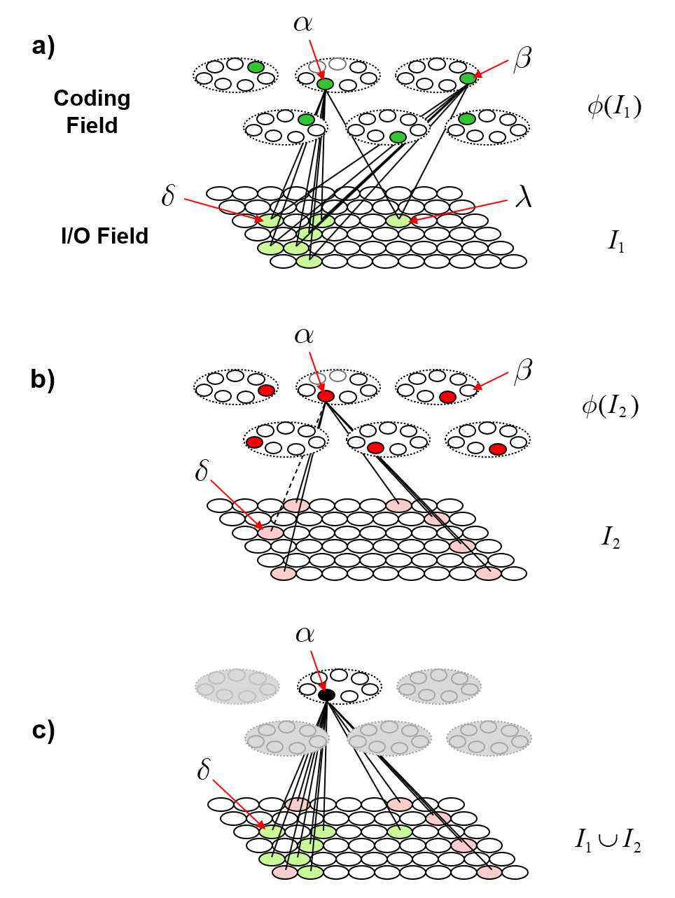
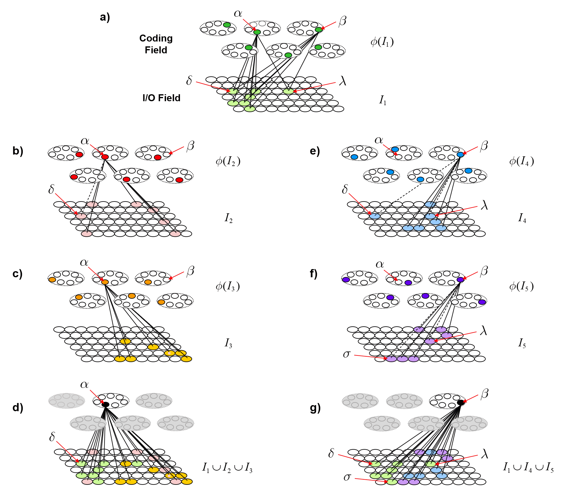
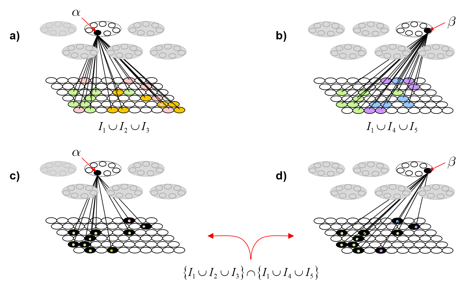
Fig. 5 now shows a more extensive example illustrating the further evolution of the same process shown in Fig. 4. In Fig. 5, we show coding unit α participating in a further code, φ(I₃), for input I₃. And we show coding unit β participating in the codes of two other inputs, I₄ and I₅, after participating, along with α, in the code of the first input, I₁. Panel d shows the final TF for α after being used in codes of three inputs, I₁, I₂ and I₃. Panel g shows the final TF for β after being used in the codes for I₁, I₄ and I₅. One can clearly see how the TFs gradually diverge due to their diverging histories of usage (i.e., interaction with the world). This corresponds to α and β becoming progressively less entangled with successive usages (interactions).

To quantify the decrease in entanglement precisely, we need to do a lot of counting. Fig. 6 shows the idea. Figs. 6a and 6b repeat Figs. 5d and 5g, showing the TFs of α and β. Figs. 6c and 6d show the intersection of those two TFs. The colored dots indicate the input from which the particular I/O unit (pixel) was accrued into the TF. In order for any future input [including any repeat of any of the learned (stored) ones] to affect α and β differently (i.e., to cause α and β to have different input sums, and thus, to have different chances of winning in their respective CMs, and thus, to ultimately cause activation of different full codes), that code must include at least one I/O unit that is in either TF but not in the intersection of the TFs. Again, all inputs are constrained to be of size S=7. Thus, after presenting any input, we can count the number of such codes that meet that criterion. Over long histories, i.e., for large sets of inputs, that number will grow with each successive input.

A storage (learning) algorithm that preserves similarity

In the examples above, the codes were chosen randomly. While we can and did provide an explanation of entanglement under that assumption, a much more powerful and sweeping physical theory emerges if we can provide a tractable mechanism (algorithm) for choosing codes in a way that statistically preserves similarity, i.e., maps similar inputs to similar codes. In this section, I will describe that algorithm. The final section will then revisit entanglement, providing further elaboration.