At the ends of papers and talks on the “learned indexes” concept described by Kraska et al in 2017, an exciting future research direction referred to as “multidimensional indexes” is suggested.

I described a multidimensional index concept about 10 years ago (unpublished) but referred to it as learning representations that were “simultaneously physically ordered on multiple uncorrelated dimensions”. The crucial property that allows informational items, e.g., records of a database consisting of multiple fields (dimensions, features), to be simultaneously ordered on multiple dimensions is that they have the semantics of extended bodies, as opposed to point masses.  Formally, this means that items must be represented as sets, not vectors.

Why is this? Fig. 1 gives the immediate intuition. Let there be a coding field consisting of 12 binary units and let the representation, or code, which we will denote with Greek letter φ, of an item be a subset consisting of 5 of the 12 units.  First consider Fig. 1a.  It shows a case where three inputs, X, Y, and Z, have been stored.  To the right of the codes, we show the pairwise intersections of the three codes.  In this possible world, PW1, the code of X is more similar to the code of Y than to that of Z.  We have not shown you the specific inputs and we have not described the learning process that mapped these inputs to these codes.  But, we do assume that that learning process preserves similarity, i.e., it maps more similar input to more highly intersecting codes.  Given this assumption, we know that

sim(X,Y) > sim(X,Z) and also that sim(Y,Z) > sim(X,Z).

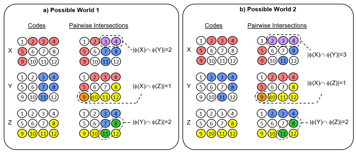
Fig. 1

That is, this particular pattern of code intersections imposes constraints on the statistical (and thus, physical) structure of PW1.  Thus, we have some partial ordering information over the items of PW1. We don’t know the nature of the physical dimensions that have led to this pattern of code intersections (since we haven’t shown you the inputs or the input space).  We only know that there are physical dimensions on which items in PW1 can vary and that that X, Y, and Z have the relative similarities, relative orders, given above.  But note that given only what has been said so far, we could attach names to these underlying physical dimensions (regardless of what they actually are).  That is, there is some dimension of the input space on which Y is more similar to X than is Z.  Thus, we could call this dimension, “X-ness”.  Y has more X-ness than Z does.  Similarly, there is another physical dimension present that we can call “Y-ness”, and Z has more Y-ness than X does.  Or, we could label that dimension “Z-ness”, in which case, we’d say that Y has more Z-ness than X does.

Now, consider Fig 1b.  It shows an alternative set of codes for X, Y and Z, that would result if the world had a slightly different physical structure.  Actually, the only change is that Y has a slightly different code.  Thus, the only difference between PW2 and PW1 is that in PW2, whatever physical dimension X-ness corresponds to, item Y has more of it than it does in PW1. That’s because |{φ(X) ∩ φ(Y)| = 3 in PW2, but equals 2 in PW1. ALL other pairwise relations are the same in PW2 as they are in PW1.  Thus, what this example shows, is that the representation has the degrees of freedom to allow ordering relations on one dimension to vary without impacting orderings on other dimensions. While it is true that this is a small example, I hope it is clear that this principle will scale to higher dimensions and much larger numbers of items.  Essentially, the principle elaborated here leverages the combinatorial space of set intersections (and intersections of intersections, etc.) to counteract the curse of dimensionality.

The example of Fig. 1 shows that when items are represented as sets, they have the internal degrees of freedom to allow their degrees of physical similarity on one dimension to be varied while maintaining their degrees of similarity on another dimension¹.  We actually made a somewhat stronger claim at the outset, i.e., that items represented as sets can simultaneously exist in physical order on multiple uncorrelated dimensions.  Fig. 2 shows this directly, for the case where the items are in fact simultaneously ordered on two completely anti-correlated dimensions.  

In Fig. 2, the coding field consists of 32 binary units and the convention is that all codes stored in the field will consist of exactly 8 active units. We show the codes of four items (entities), A to D, which we have handpicked to have a particular intersection structure.  The dashed line shows that the units can be divided into two disjoint subsets, each representing a different “feature” (latent variable) of the input space, e.g., Height (H) and IQ (Q).    Thus, as the rest of the figure shows, the pattern of code intersections simultaneously represents both the order, A > B > C > D, for Height and the anti-correlated order, D > C > B > A, for IQ.

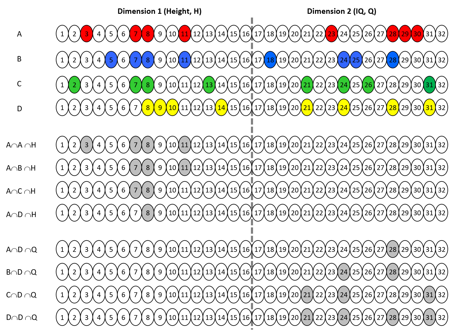
Fig. 2

The units comprising this coding field may generally be connected, via weight matrices, to any number of other, downstream coding fields, which could “read out” different functions of this source field, e.g., access the ordering information on either of the two sub-fields, H or Q.

The point of these examples is simply to show that a set of extended objects, i.e., sets, can simultaneously be ordered on multiple uncorrelated dimensions.  But there are other key points including the following.

1. Although we hand-picked the codes for these examples, the model, Sparsey, which is founded on using a particular format of fixed-size sparse distributed representation (SDR), and which gave rise to the realization described in this essay, is a single-trial, unsupervised learning model that allows the ordering (similarity) relations on multiple latent variables to emerge automatically.  Sparsey is described in detail in several publications: 1996 thesis, 2010, 2014, 2017 arxiv.
2. While conventional, localist DBs use external indexes (typically trees, e.g., B-trees, KD-trees) to realize log time best-match retrieval, the set-based representational framework described here actually allows fixed-time (no serial search) approximate best-match retrieval on the multiple, uncorrelated dimensions (as well as allowing fixed-time insertion).  And, crucially, there are no external indexes: all the “indexing” information is internal to the representations of the items themselves.  In other words, there is no need for these set objects to exist in an external coordinate system in order for the similarity/ordering relations to be represented and used.

Finally, I underscore two major corollary realizations that bear heavily on understanding the most expedient way forward in developing “learned indexes”.

1. A localist representation cannot be simultaneously ordered on more than one dimension.  That’s because localist representations have point mass semantics.  All commercial DBs are localist: the records of a DB are stored physically disjointly.  True, records may generally have fields pointing to other records, which can therefore be physically shared by multiple records.  But any record must have at least some portion that is physically disjoint from all other records.  The existence of that portion implies point mass semantics and (ignoring the trivial case where two or more fields of the records of a DB are completely correlated) a set of points can be simultaneously ordered (arranged) on at most one dimension at a time.  This is why a conventional DB generally needs a unique external index (typically some kind of tree structure) for each dimension or tuple on which the records need to be ordered so as to allow fast, i.e., log time, best-match retrieval.
2. In fact, dense distributed representations (DDR), e.g., vectors of reals, as for example present in the internal fields of most mainstream machine learning / deep learning models, also formally have point mass semantics.  Intersection is formally undefined for vectors over reals.  Thus, any similarity measure between vectors (points) must also formally have point mass semantics, e.g., Euclidean distance.  Consequently, DDR also  precludes simultaneous ordering on multiple uncorrelated dimensions.

Fig. 3 gives final example showing the relation of viewing items in terms of a point representation to set representation.  Here the three stored items are purple, blue, and green.  Fig. 3a begins showing the three items as points with no internal structure sitting in a vector space and having some particular similarity (distance) relationships, namely that purple and blue are close and they are both  far away from green.  In Fig. 3b, we now have set representations of the three items.  There is one coding field here, consisting of 6×7=42 binary units and red units show intersection with the purple item’s representation. Fig 3c shows that the external coordinate system is no longer needed to represent the similarity (distance) relationships, and Fig. 3d just reinforces the fact that there is really only one coding field here and that the three codes are just different activation patterns over that single field. The change from representing information formally as points in an external space to representing them as sets (extended bodies) that require no external space will revolutionize AI / ML.

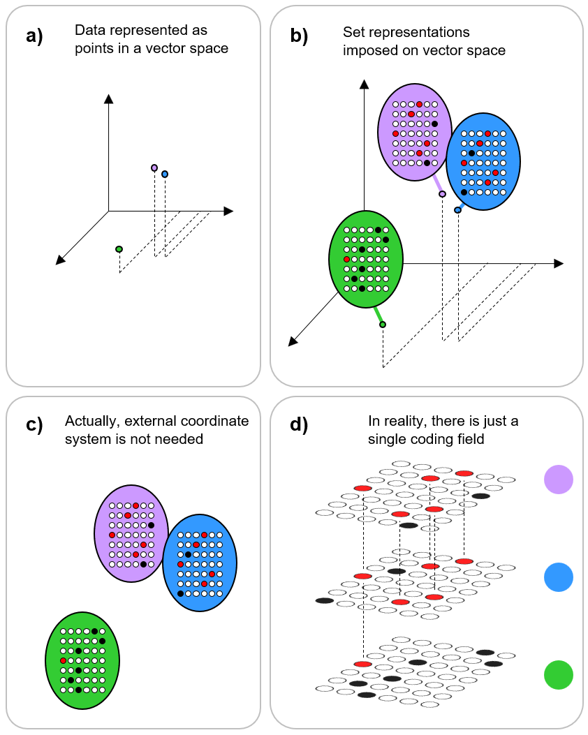
 Fig. 3