The Classical Realization of Quantum Parallelism

In this essay, I’ll explain how quantum parallelism can be achieved on a classical machine.  Quantum parallelism is usually described as the phenomenon in which a single physical operation, e.g., the execution of a Hadamard gate on an N-qubit memory of a quantum computer, physically affects (updates) the representations of multiple entities, e.g., of all 2N basis states held in quantum superposition in the N-qubit memory.1  This is the source of the idea that quantum computation is exponentially faster than classical computation.  It seems that almost no one working in quantum computing believes quantum parallelism is realizable on classical hardware, i.e., with plain old bits.  I believe this is due to the implicit assumption of localist representation in the mathematical formalism, inherited from quantum mechanics, which underlies mainstream quantum computing approaches.2

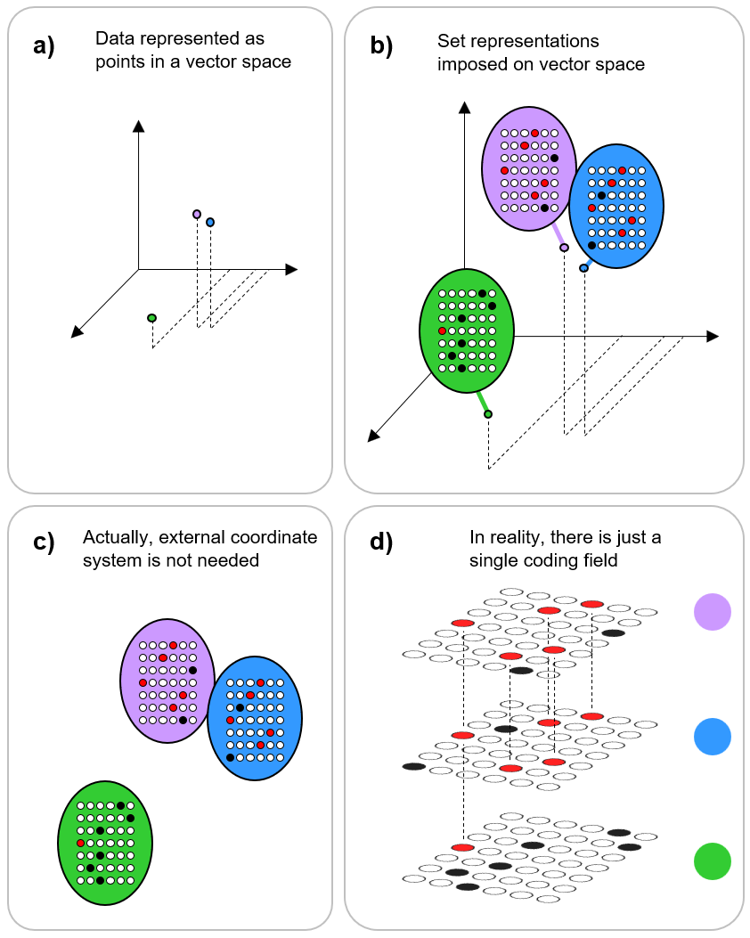
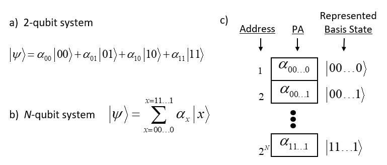
A localist representation is one in which each represented entity is represented by its own distinct representational unit (hereafter “unit” when not ambiguous), i.e., disjoint from the representations of all other entities.  The localist representation present in quantum computing is clear in Figure 1.  The 2-qubit system of Fig. 1a has 22=4 basis states.  Each state is represented by its own symbol, e.g., |00⟩, with its own complex-valued probability amplitude (PA), e.g., α00.  Fig. 1b gives the expression for an N-qubit system, which has 2N basis states (assume index var, x, has N places).  Figure 1c shows a localist representation of the PAs, and thus, effectively, of the basis states themselves, of the N-qubit system, stored in a classical computer memory. Each PA resides in its own separate physical memory location. Therefore, performing a physical operation on any one PA, e.g., the physical act of changing one of its bits, produces no effect on any of the other 2N-1 PAs.  I believe that this localist assumption apparent in Fig. 1c is what underlies the virtually unanimous opinion that simulating quantum computation on a classical machine takes exponential resources, both spatially (number of memory locations) and temporally (number of atomic operations needed). 

Formal representation of a 2-qubit system and how the probability amplitudes (PAs) are all stored in distinct memory locations when they are represented localistically in a classical memory
Figure 1: Localist Nature of the Formalism of Quantum Mechanics and Mainstream Quantum Computing.

The “Quantum Leap” in Computing is a Change of Representation, not Hardware

If, instead of localist representations, entities are represented by distributed, and more specifically, sparse distributed, representations (hereafter SDRs), then the power of quantum computation—specifically, quantum parallelism—can be achieved with sub-exponential resources, both in space and time, on a classical machine.  As we will see, this is because when entities are represented as SDRs, plain old classical superposition, i.e., representing entities as sets, specifically, sparse sets,of physical objects, i.e., of classical bits, which can intersect, provides the capability described as quantum parallelism.

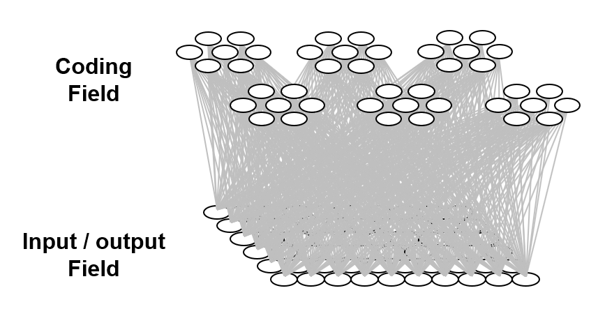
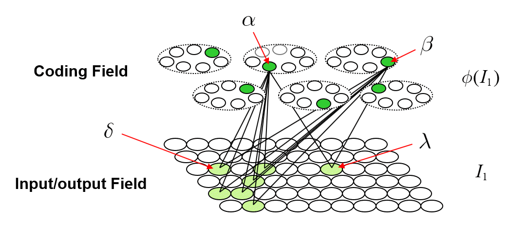
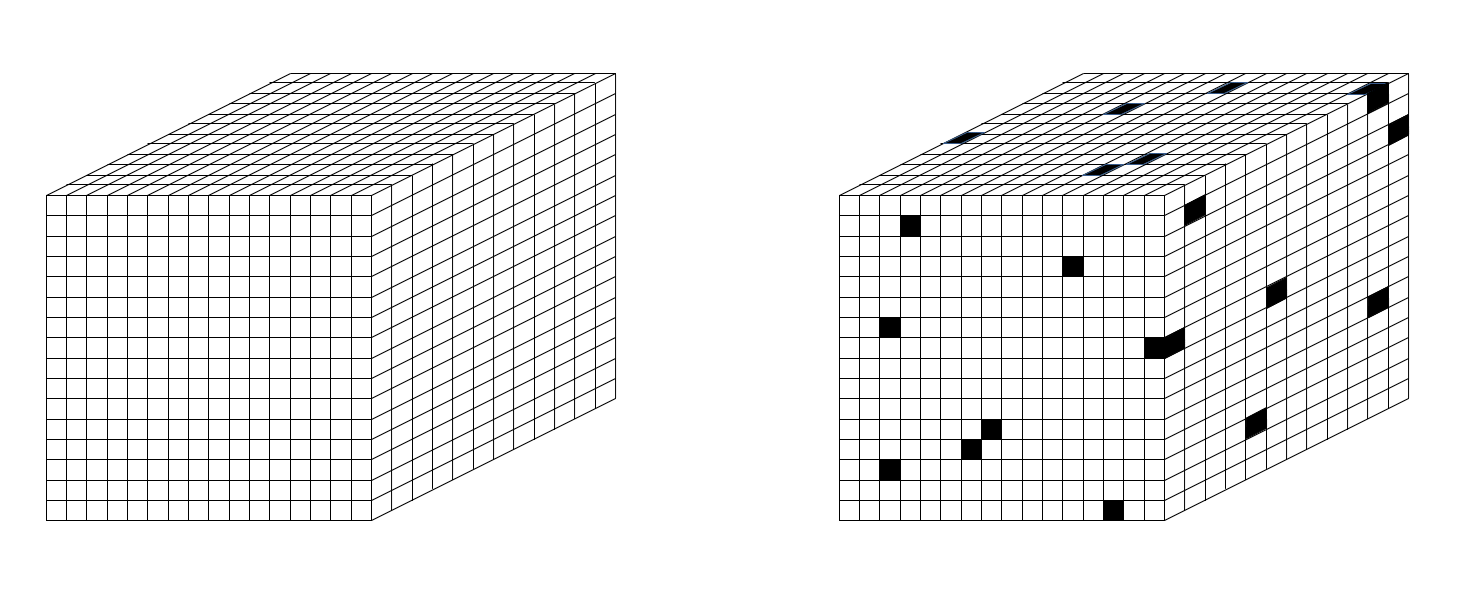
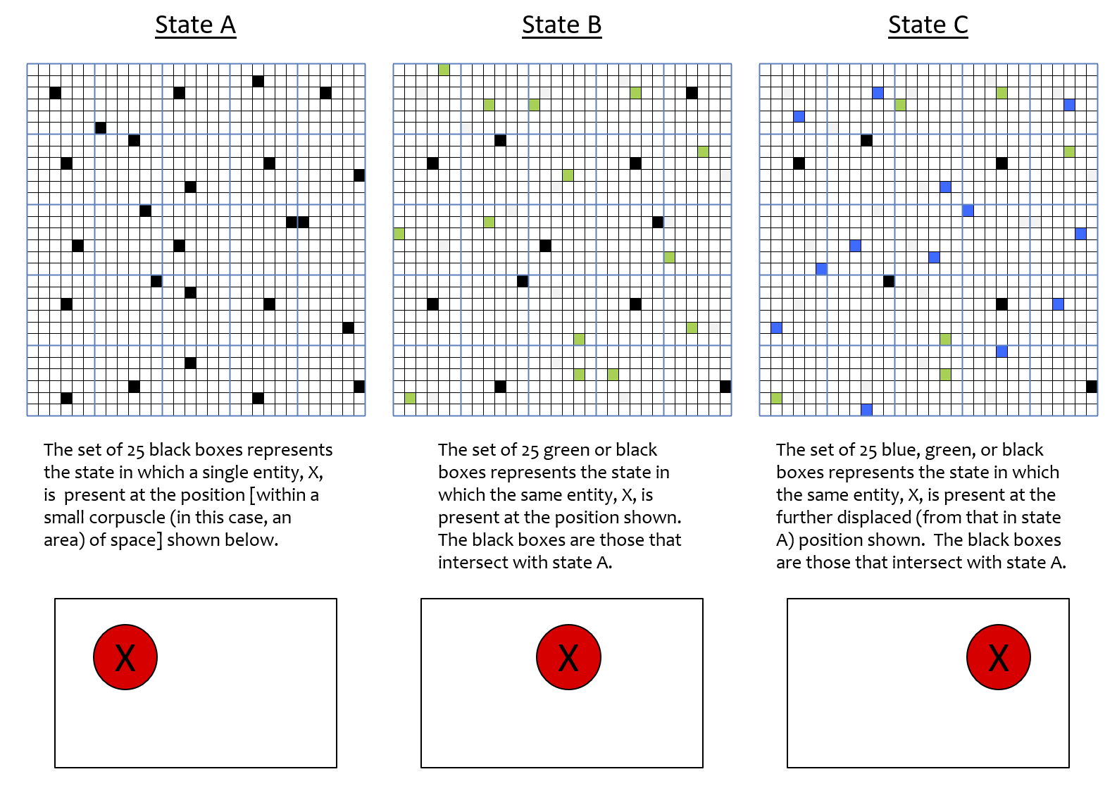
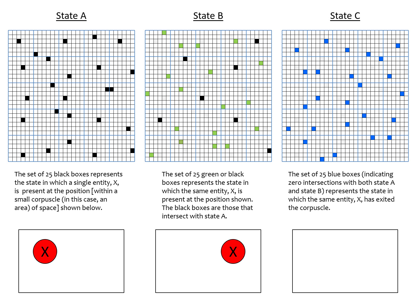
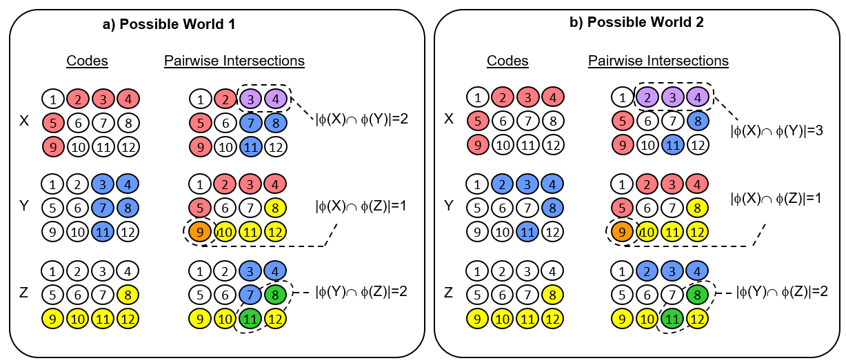
In particular, the SDRs in the model I’ll be describing, Sparsey (1996, 2010, 2014, 2017), are small sets of binary units chosen from a much larger “coding field“, where these SDRs (sets) can intersect to arbitrary degrees.  This raises the possibility of using the size of intersection of two SDRs to represent the similarity of the entities (items) they represent.  We’ll refer to this property as similar-inputs-to-similar-codes, or “SISC” (n.b.: “code” is synonymous with “representation”).   Fig. 2 shows the structure of a Sparsey coding field. Fig. 2a shows one in a linear format: it is a set of Q winner-take-all (WTA) competitive modules (CMs) (red dashed boxes), each consisting of K binary units. Here, Q=7 and K=7 (in general, they can be different).  A particular code, consisting of Q active (black) units, one in each CM, is active in the field. N.b.: All codes stored in this field will be of the same size, Q.  The total number of unique codes that can be represented, the codespace, is KQ.3 Fig. 2b shows a 3D view of the field in hexagonal format.  It also shows an 8×8 input field of binary pixels, which is fully (completely) connected to the coding field via a binary weight matrix (blue lines).  Fig. 2c shows an example active input, A (e.g., a small visual line/edge ), an active code, φ(A), chosen to represent A, and the weights (blue lines) that would be increased (from 0 to 1) from the active input pixels to active coding units, to store A.

fig_2_blog
Figure 2: Structure of a Sparsey SDR coding field.

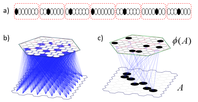
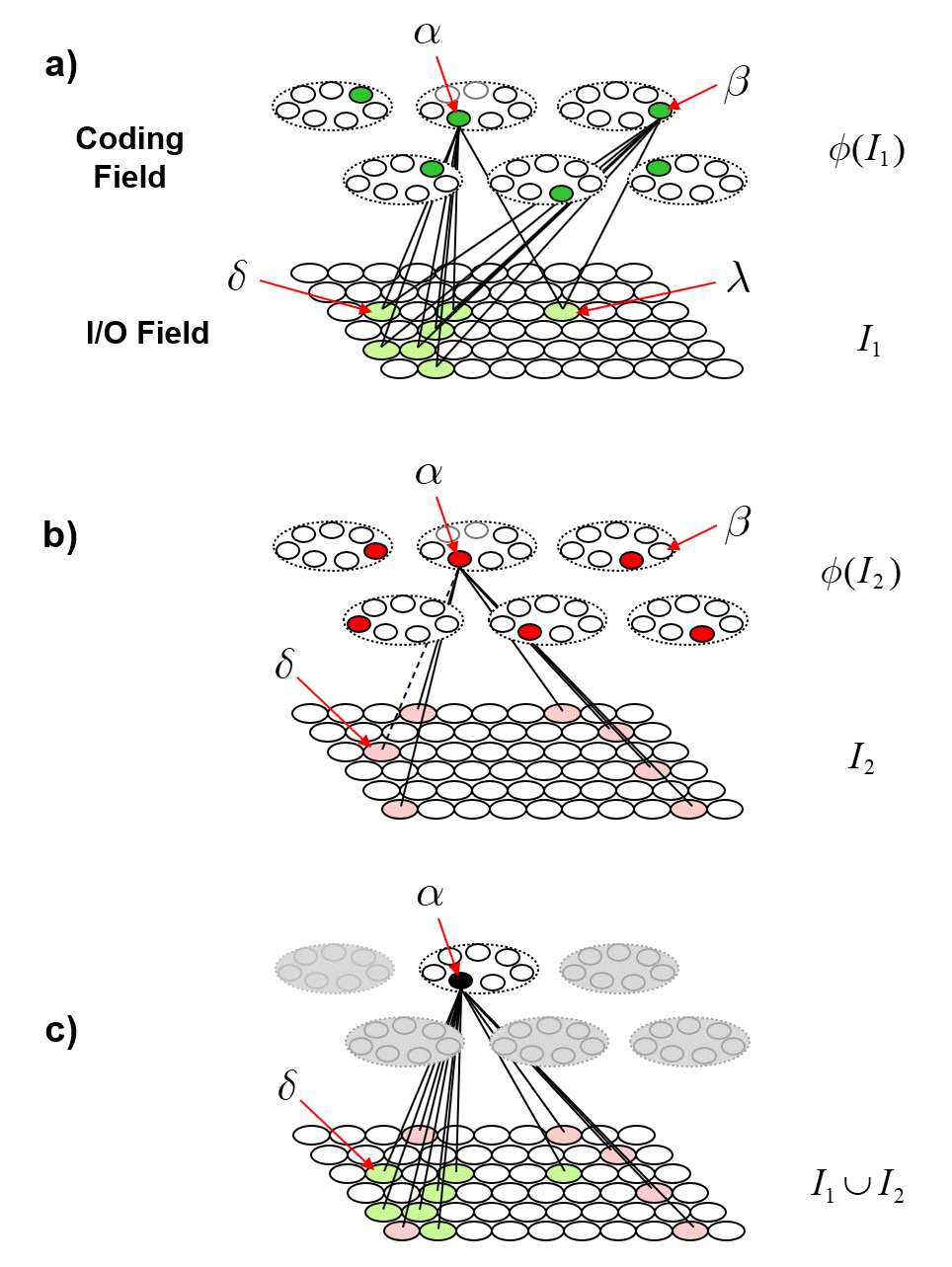
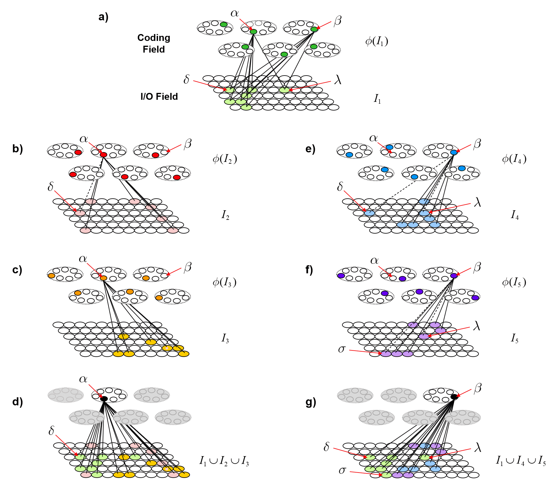
Figure 3 (below) illustrates the basis for quantum parallelism in a Sparsey SDR coding field. The top row shows the notional input, A , and corresponding SDR (Code), φ(A), from Fig. 2c. The next four rows then show progressively less similar inputs (measured as pixel overlap), B-E, and corresponding SDRs, φ(B)-φ(E), which were manually chosen to exemplify SISC. The second and last columns show that code similarity, measured as intersection, correlates with input similarity. Note that while the codes were manually chosen in this example, Sparsey’s unsupervised learning algorithm, the Code Selection Algorithm (CSA) (summarized in this section) finds such SISC-respecting codes in fixed-time. The bottom row (below dashed line of Fig. 3) then reveals the following crucial property.

Whenever any ONE particular code is fully active, i.e., all Q of its units are active, ALL other codes stored in the field will also be simultaneously physically active with degree (i.e., strength) proportional to their intersections with the single fully active code.

The likelihood (unnormalized probability) of a basis state is represented by the fraction of its code’s units that are physically active, i.e., by a set of co-active physical units. This contrasts fundamentally to quantum mechanics in which the probability of a basis state is represented by complex number.

For example, the leftmost chart shows that when φ(A) is fully active, φ(B)-φ(E) are active with appropriately decreasing strength. And similarly, when any of the other four codes is fully active (the other four charts). I emphasize that the modular organization of the coding field, i.e., the division of the overall coding field into Q winner-take-all (WTA) modules, is very important. As described here, it confers computational efficiencies over any “flat field” implementation of SDR (as in Kanerva’s SDM model and its various descendants, e.g., Numenta’s HTM). In addition, Sparsey’s WTA module has a clear possible structural analog in the brain’s cortex, i.e., the minicolumn (as discussed in Rinkus 2010). One manifestation of the exponential increase in computational efficiency provided by SDR (assuming the learning algorithm preserves similarity) was previously described in this 2015 post.

SDR_SISC_fig
Figure 3:   With SDR, All Stored Codes Are Simultaneously Physically Active in Classical Superposition. Figure adapted from 2012 paper.

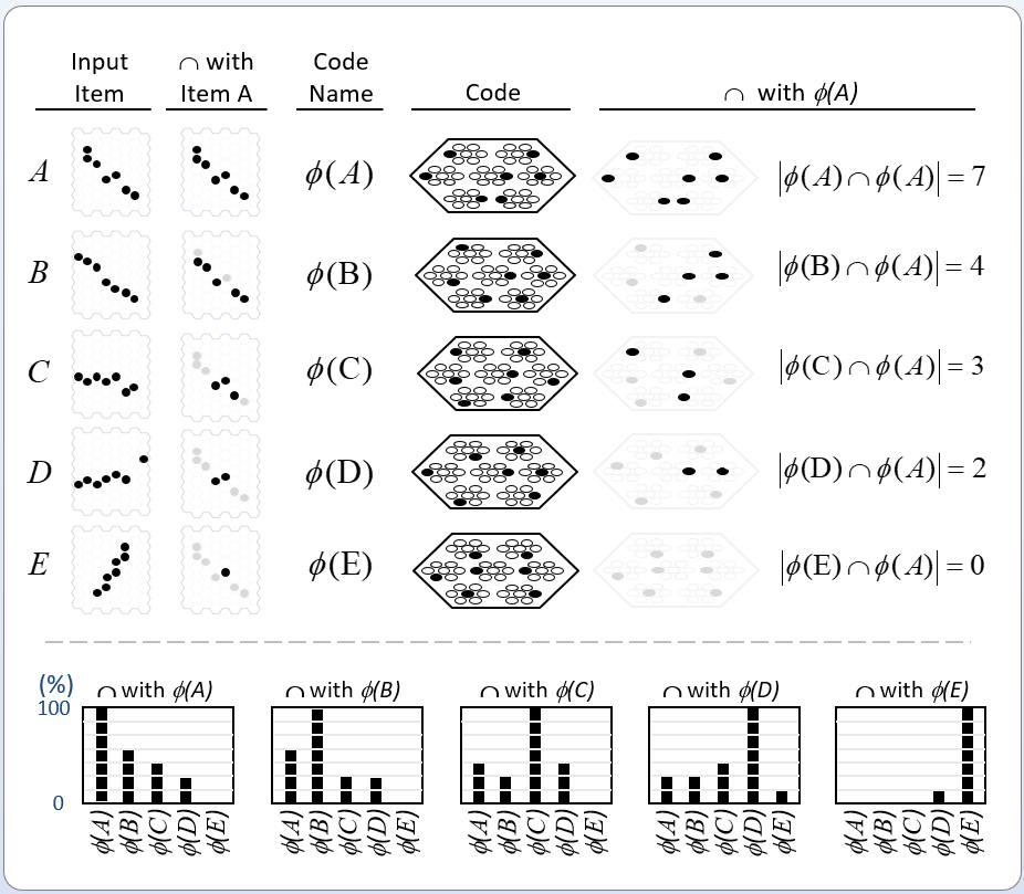
We must take some time to dwell on the property shown in Fig. 3 (and stated in bold above) because it’s really at the heart of this essay and of my argument. It shows that when entities, e.g., basis states, are formally represented as sets, as opposed to vectors (as is the case in quantum mechanics),

purely classical superposition provides the functionality of quantum superposition.

What do I mean by this? Well first, consider Copenhagen, the prevailing interpretation of quantum mechanics (hereafter “QM“). It says that at every moment, ALL basis states of a physical system exist simultaneously in quantum superposition and that there is a probability distribution over those states giving the probability that each particular state would be observed if the system is observed. So that’s the functionality of quantum superposition: allowing ALL physical states to exist in the same space at the same time, with a probability distribution over the states.

The problem is that Copenhagen has never, in a 100 years (!), provided a physical explanation of how multiple different physical states can exist in the same space at the same time. Instead, they have been forced to assert that the probability distribution, which is formally a mathematical, not a physical object, is somehow more physically real than the physical basis states themselves.

Now consider what’s being shown in Fig. 3. It’s purely classical. The individual units are bits, not qubits. Yet, as the charts at bottom of the Fig. 3 show, whenever any one code is active, ALL stored codes are simultaneously proportionally physically active. This constitutes a physically straightforward and immediately apparent explanation of how multiple, in fact, ALL, stored codes, can simultaneously physically exist in the same space, where here, the “space” is the (physically instantiated) SDR coding field. We underscore three keys to this explanation.

  • The codes (SDRs) are highly diffuse (sparse).
  • The SDRs are formally sets comprised of multiple (specifically, Q) atomic physical units (the binary units of the coding field), or in other words, they are “distributed”. This is essential because it admits a straightforward physical interpretation of what it means for a stored code to be partially active, namely that a code is active with strength proportional to the fraction of its Q units that are active.4
  • Every code is spread out, again diffusely, throughout the entire coding field. This is enforced by the modular structure of the coding field, i.e., the fact that it is broken into Q WTA modules and every SDR must consist of one winner in each module.5

To be sure, in Fig. 3, we’re talking about classical superposition of codes, in particular, of SDRs, which represent physical states (e.g., basis states of an observed system), not about superposition of the physical states themselves. So, we’re not, in the first place, in the realm of QM per se, which was developed as an explanation of physical reality, i.e., of physical objects/systems, and their dynamics, irrespective of whether or not such objects/systems represent information. However, we are exactly in the realm of quantum computing. That is, a quantum computer, like any classical computer, is a physical system for representing and processing informational objects. In a quantum computer, as in any classical computer, it is representations of states (of some other system, e.g., of entries in a database, of states of some simulated physical system, e.g., a system of molecules) and representations of their transitions (dynamics), not the states/transitions themselves, that are physically reified (e.g., in memory).

At the outset, I asserted that the essential problem with mainstream quantum computing is that the founders of QM and of quantum computing were thinking as “localists”. But from another vantage point, the essential problem was the original formalization of QM in terms of vector spaces, specifically Hilbert spaces, rather than sets. In QM, all entities (and compositions of entities, i.e., entities of any scale, from fundamental particles to macroscopic bodies) are formally vectors, and thus are formally equivalent to points, i.e., have the semantics of entities with zero extension. As such it is immediately clear that there can be no formal concept of graded degrees of intersection of entities in QM.6 It is therefore not surprising that none of the founders of QM, Bohr, Heisenberg, Schrodinger, Born, Dirac—who were all thinking in terms of a vector-based (thus, point-based) formalism—ever developed any physically intuitive (commonsense) explanation of how multiple entities (world states) could simultaneously be partially active (i.e., at different graded levels/strengths) in the same space. This most fundamental of axioms, adopted by QM’s founders, to represent physical entities as vectors, i.e., 0-dimensional points, is precisely what prevented any of those founders from seeing, apparently from ever even entertaining the idea, that classical superposition can provide the full functionality of quantum superposition, and thus can realize can realize what is termed quantum parallelism in the language of QC.  But as explained here (most pointedly, with respect to Fig. 3, but throughout), in the realm of information processing, when entities (informational objects) are formally represented as sets, partial (graded) degrees of existence have an obvious and simple classical physical realization (again, as just the fraction of the elements of the set representing an entity that is active). I predict that this change—from vectors to sets, and from localist representations to SDRs—will constitute a “sea change” for quantum computing, and by extension for QM. For yet other implications of the difference between representing entities formally as sets vs vectors, see my earlier post on Learning Multidimensional Indexes”.

More on the Relation of Quantum Parallelism to the Localist vs. Distributed Representation Dichotomy

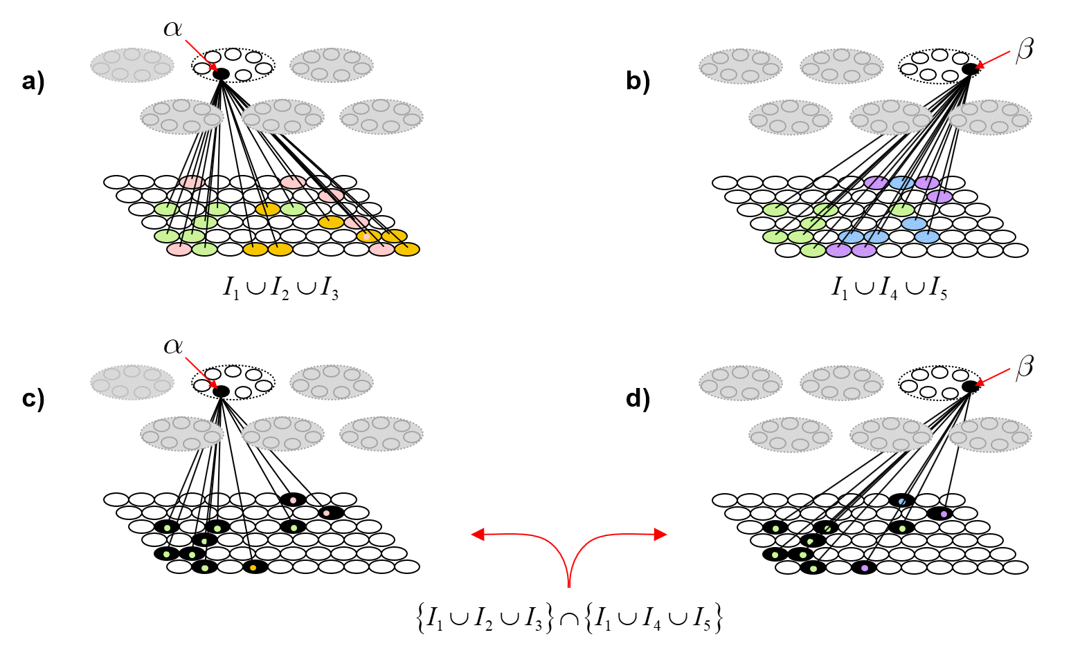
Figure 4 revisits Fig. 1 to further clarify why localist representations preclude quantum parallelism. The upper left portion recapitulates Fig. 1 (with a minor change of indexing of units from 1-based to 0-based) and adds an explicit depiction of the memory block for a bottom-up weight matrix (red dashed box) from the input field (for simplicity, the input units are assumed to be binary). We assume the matrix is complete and since the internal representational (i.e., coding) field (black dashed box) is localist, that matrix has M x 2N weights. The lower middle portion shows the coding field, now denoted A, again, and where, for concreteness, we assume there are N=3 input units. Thus, there are 23=8 possible input (basis) states and each has its own memory location. We show a particular probability distribution over those states at time t: the values sum to 1, and |100⟩ is most likely. We then introduce another matrix (green), a recurrent matrix that completely connects A to itself. The idea is that signals originating at time t recur back to A at t+1 whereupon some processing occurs in the coding field (in particular, including all 23 units computing their input summations), resulting in an updated probability distribution over the states at t+1. This recurrent matrix is 2N x 2N, and corresponds to a unitary operator of QM, and this will be discussed further in relation to Fig. 5. The red boxes identify the two essential weaknesses of localist representations with respect to quantum parallelism. First, as pointed out in the lower red box, and as stated at the outset, applying a physical operation on any one memory location, changes the value of only the one basis state represented by that location. Consequently, updating all 2N basis states requires 2N physical operations. Second, as pointed out in the upper red box, applying a physical operation to change the signal value on any one (bolded green line) of the 2N x 2N recurrent connections (or to change the weight of the connection) affects only the one basis state at the terminus of that connection. Clearly, it is the localist representation per se, that precludes the possibility of quantum parallelism.

Explanation of why localist representations preclude quantum parallelism
Figure 4: Explanation of why Localist Representations Preclude Quantum Parallelism

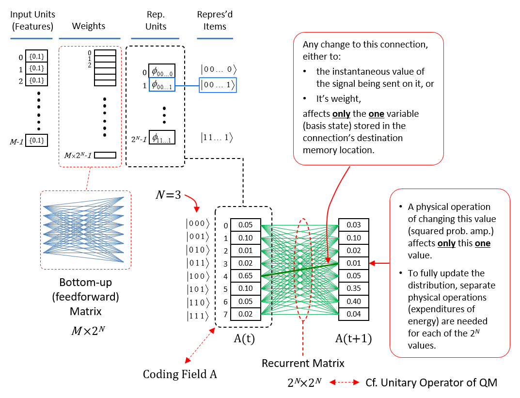
Figure 5 now shows the physical realization of quantum parallelism when items are represented as SDRs. As the “Representational Units” column shows, in the SDR case, the coding field is now organized as Q blocks of memory [the competitive modules (CMs) described above], each with K memory locations (which, in this case, can literally be just single bits), for a total of QK locations. Again, assuming N=3 input units, the next column shows the 23 represented items, i.e., basis states, and the colored lines between the columns show (notionally) the SDRs of three of the represented states. The blue arrows show that the code of |000⟩, φ(|000⟩), consists of the second unit in CM q=0, the second unit in CM q=1, …, and the last unit in CM, q=Q-1. The red arrows show the code for |110⟩, φ(|110⟩), which intersects with φ(|000⟩) in CM q=1, and so forth. The bottom right portion of the Fig. 5 shows the coding field again, where for concreteness, Q=5 and K=3, and shows the completely connected recurrent matrix (green). Note in particular, that the number of weights, (QK)2, in the recurrent matrix no longer depends on the number of represented (stored) basis states as for the localist case in Fig. 4. To the right, we see three possible states of the coding field, i.e., concrete codes for the three (out of 23) basis states above.

Explanation of how SDR Realizes Quantum Parallelism
Figure 5: Explanation of how SDR Realizes Quantum Parallelism

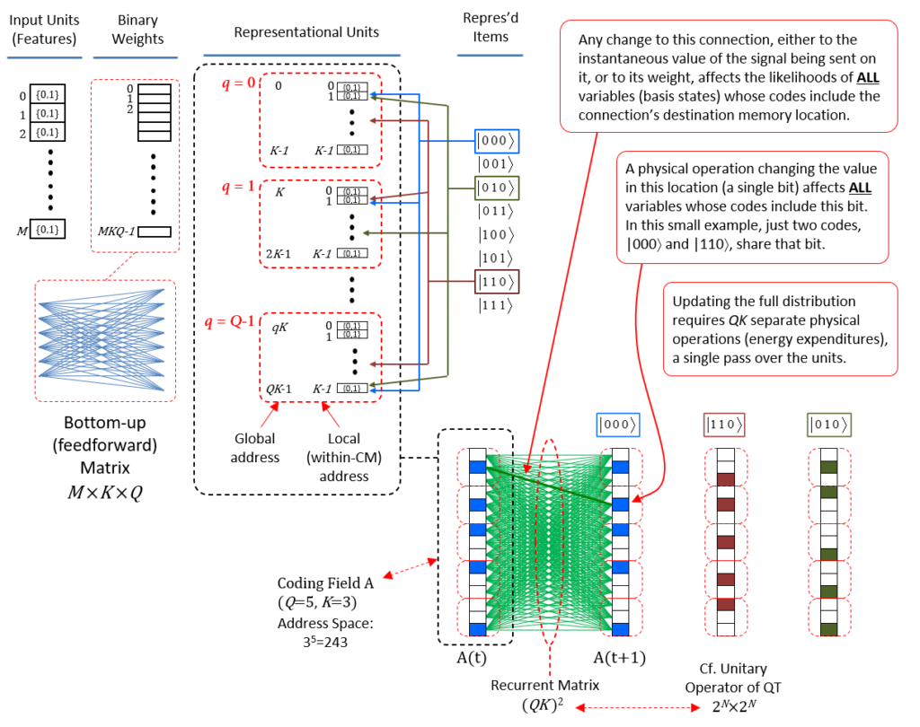
The red boxes of Fig. 5 explain how quantum parallelism is realized in the case of SDR. The middle red box explains that when a physical operation is applied to any one unit of the coding field, in particular, the second unit of CM 1 (red arrow), ALL represented basis states whose SDRs include that unit are necessarily changed. For example, if the operation turns this unit off, then not only is the state, |000⟩, less strongly present, but so is the state, |110⟩: a single expenditure of energy at a particular point in space, a single bit, physically updates the states of multiple represented entities, i.e., quantum parallelism. This example clearly shows that using SDR implies quantum parallelism.7 The lower red box then explains that making a single pass over the QK memory locations, thus, QK physical operations, necessarily updates the full distribution over all stored codes. The crucial question is then: how many SDRs can be stored in such a field, or more specifically, how does the number of codes (i.e., of represented basis states of some observed/modeled system) that can be safely stored grow as a function of QK? As described below (Fig. 9), the results from my 1996 PhD thesis show that that number grows super-linearly in QK.

Finally, the upper red box of Fig. 5 explains that applying a single physical operation to any one connection (weight) necessarily affects ALL SDRs that include the unit at the terminus of that connection: again, this is quantum parallelism, but operating at the finer scale of the weights as opposed to the units. For example, if the weight of the bold green connection is increased (assume real-valued wts for the moment), then the input summation to its terminus unit (second unit in CM 1) will be higher. Since the CM functions as a WTA module, where the winner is chosen as a draw from a distribution (a transformed version of the input summation distribution), that unit will then have a greater chance of winning in CM 1. Thus, every SDR that includes that unit will have a greater likelihood of being activated as a whole, all from a single physical operation applied to a single memory location (representing a single weight). [The algorithm is summarized below.]

The Recurrent Matrix Embeds State Transitions that are Analogs of Unitary Operators of QM

I said above that the recurrent matrix corresponds to a unitary operator of QM. More precisely, the recurrent matrix is a substrate in which (in general, many) operators are stored, i.e., learned, during the unsupervised learning process. However, note that in QM, an operator is the embodiment of physical law (i.e., time-dependent Schrodinger equation) and is NOT viewed as being learned. Moreover, the approach of mainstream quantum computing has largely been to DESIGN operators, i.e., quantum gates and circuits composed of such gates, which perform generic logical operations; again, no learning.

Therefore, in yet another major departure from quantum mechanics and from mainstream quantum computing, in the machine learning (specifically, Sparsey’s unsupervised learning) scenario described here, the operators ARE learned from the data.

To flesh this out, let’s consider the case where the inputs are spatiotemporal patterns, e.g., sequences of visual frames as in Fig. 6. The figure shows a Sparsey coding field (rose hexagon), comprised of Q=7 WTA CMs, each composed of K=7 binary units, experiencing three successive frames of video of a translating edge in its input field, i.e., its “receptive field” (green hexagon). The coding field chooses an SDR (black units) for each input on-the-fly as it occurs and increases, from 0 to 1, all recurrent weights from units active at T to units active at T+1 (green arrows, and only a tiny representative sample shown, and in general, some may already have been increased by prior experiences).8. Thus, input sequences are mapped to chains of SDRs (further elaborated on here, here, here, and most thoroughly, in my 2014 paper).

Figure 6: Memories of Sequences as Chains of SDRs

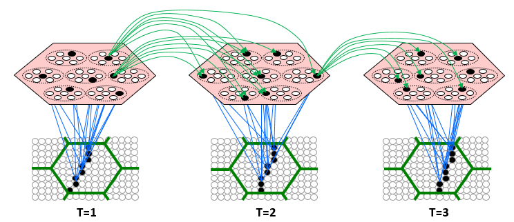
Fig. 6 depicts Sparsey’s primary concept of operations, i.e., to automatically form such SDR chains (memory traces) in response to the input sequences it experiences. But consider just a single association formed between one input frame and the next, e.g., between T=1 and T=2 of Fig. 6. This association, which is just a set of increased binary weights, can be viewed as an operator. It’s an operator that is formed, with full strength based on the single occurrence of two particular, successive states of the underlying physical world. From the vantage point of traditional statistics, this is just one sample and in general, we would not want to embed a memory trace of this at full strength: after all, it could be noise, e.g., it could reflect accidental alignments of one of more underlying objects and thus not reflect actual (or in any case, important) causal processes in the world. Nevertheless, Sparsey is designed to do just that, i.e., to embed this state transition as a full strength memory trace based on its single occurrence.9 It’s true that such an operator (state transition) is therefore highly idiosyncratic to the system’s specific experiences. However, because:

  1. all such state-to-state transitions, which again are physically reified as sets of changed synaptic weights, are superposed (just as the SDRs themselves are superposed), and
  2. Sparsey’s algorithm for choosing SDRs, the Code Selection Algorithm (CSA), preserves similarity (see below)

subsets of synapses that are common to multiple individual state-to-state transitions come to represent more generic causal and spatiotemporal similarity relations present in the underlying (observed) world. Hence, Sparsey’s dynamics realizes the continual superposing of operators of varying specificities directly on top of each other. Many/most of the more specific ones (akin to episodic memories) will fade with time, leaving the more generic ones (akin to semantic memories) in their wake.

Finally, what about the unitarity requirement of QM’s operators? That is, QM allows only unitary operators, i.e., operators that preserve a norm. This is required because the fundamental entity of QM is the probability distribution that exists over the basis states of the relevant physical system. Thus, in QM, all physical actions MUST result in a next state of the physical world that is also characterized by a probability distribution, i.e., must preserve the L2 norm to be of length 1. However, as noted above, e.g., with respect to Fig. 3, the instantaneous state of a Sparsey coding field, which is always a set of Q active binary units, represents a likelihood distribution over the stored codes. The likelihoods are fractions between 0 and 1, but do not sum to 1. Indeed, the total sum of likelihoods will in general change from one time step to the next. Of course, the vector of likelihoods over the stored codes can in principle, always be normalized (by dividing them all by the sum of all the likelihoods) to produce a true probability distribution. However, Sparsey’s update dynamics (see next section) effectively achieves this renormalization without requiring that explicit computation.

Summary of Sparsey’s Code Selection Algorithm (CSA)

The key innovation of Sparsey is a simple, general, single-trial (one-shot), and most importantly, “fixed-time” unsupervised learning (storage) algorithm, the Code Selection Algorithm (CSA), which preserves similarity from the input space to the code (SDR) space, i.e., maps more similar inputs to more similar, i.e., more highly intersecting, SDRs.10 Fig. 7 illustrates this algorithm. The example involves a tiny instance of a Sparsey coding field comprised of Q=5 WTA CMs, each with K=3 units, and which receives a complete binary matrix (all wts initially 0, light gray) from an input field having 8 binary units. The top panel (at left) shows the four inputs, A to D, that will be considered. Note that we constrain all inputs to be of the same size, i.e., 5 active units, and that inputs B to D are progressively less similar to A. In the top panel (center), we show the act of learning input A: A is presented, an SDR, φ(A), is chosen by randomly picking a winner in each CM, and all weights from active input units to active coding units are increased from 0 to 1 (a simple Hebbian learning rule). A is the only input that will be learned in this example: the remaining four panels (1-4) illustrate the cases of presenting A, B, C, or D, as a test input, after having learned only A.

While the text in the Fig. 7 fully explains the dynamics, I’ll walk through it in the text here too. In Panel 1, we present A again. Due to the learning that occurred in the learning trial, the bottom-up (u) input sum will be u=5 for the five units that were randomly chosen to be in φ(A) and u=0 for all other units (shown in the yellow bar charts above the CMs). Clearly, if this model is being used as an associative memory, we would want the code originally assigned to this input, φ(A), to be activated exactly again. That would constitute the model recognizing the input. In this particular case, the model could achieve this by simply activating the unit with the hard max input sum (u) in each CM. However, for reasons that will be made clear in the remaining panels, Sparsey works differently. Rather, what Sparsey does is transform the u vector in each CM into a probability (ρ) distribution and then draw the winner from that distribution (i.e., a soft max in each CM).11 Here for example, the transform applied in each CM gives a little probability to each of the u=0 units, but most to the u=5 unit.12 In other words, the u distribution is slightly compressed (flattened, whitened) to yield the ρ distribution. In this case, we expect the max-ρ unit to win in most of the CMs, but lose occasionally (an exact expectation could be computed as a Bernoulli distribution, but that detail is not important to illustrate the essential concept of the algorithm). For argument’s sake, in this case, we show the max-ρ unit actually being chosen in all Q CMs, i.e., perfect reactivation of φ(A).

Figure 7: Simplified Explanation of how Sparsey Preserves Similarity

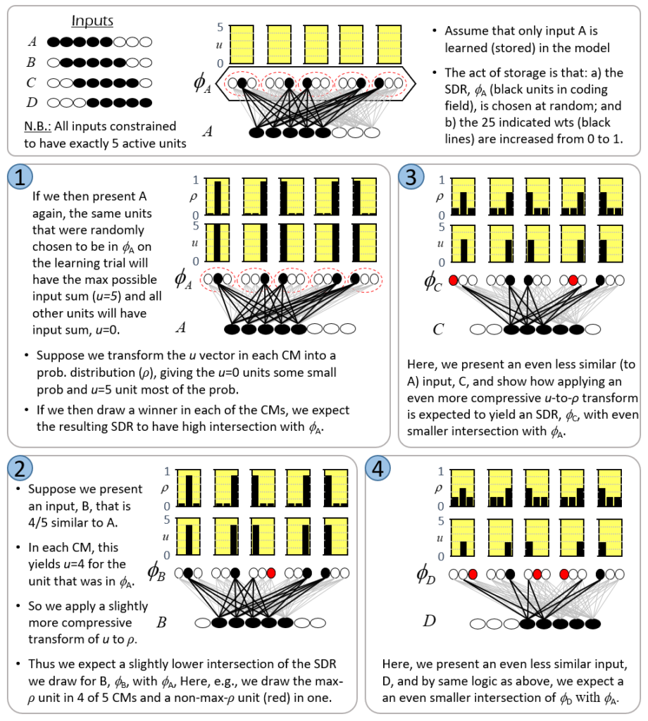
In Panel 2, we present a novel input, B, which is very, i.e., 4/5, similar to A. In fact, the model cannot know whether B is a truly novel input, i.e., whether its featural difference from A has important consequences and thus, whether B should be stored as a unique input, or whether B is a just a noisy version of A, in which case, A’s code, φ(A), should just be reactivated exactly. This is a meta-question (addressed for example in my 1996 thesis), but for the sake of this example, let’s assume it’s a truly novel input. In this case, despite the fact that we want to assign a unique code, φ(B), to B, we nevertheless should want φ(B) to be similar to φ(A), which in the case of SDRs, means having a high intersection. Following the reasoning given for Panel 1, we can achieve this result, i.e., approximately preserve similarity, by simply applying a slightly more compressive transform of u to ρ distributions in each CM (i.e., assign slightly more probability of winning to the u=0 units than in Panel 1, but still, much more probability of winning to the u=5 unit), as shown in Panel 2. For argument’s sake, we show the max-ρ unit winning in 4 out of 5 CMs, and the non-max-ρ unit (red unit) winning in one CM. Thus, B is 80% similar to A, and φ(B) is 80% similar to φ(A). The fact that the input and code similarities are both 80% here is incidental. What’s important is just this general principle that if we simply make the degree of compression of the u-to-ρ transform be inversely related to input similarity (directly proportional to novelty), we will approximately preserve similarity. Panels 3 and 4 just illustrate the same reasoning applied to progressively less similar inputs as the figure’s text explains. Hopefully, it is now clear why winners must be chosen using soft max rather than hard max: if hard max was used to pick the winner in each CM in panels 2-4 of Fig. 7, then the same exact SDR would be assigned to all four inputs. If the goal is to ensure (approximately) SISC, then soft max must be used.

Fig. 7 illustrates the essential concept of Sparsey’s Code Selection Algorithm (CSA), which can be described simply as: adding noise into the process of selecting winners (in the CMs), the magnitude (power) of which varies directly with the novelty of the input. Or, we can describe this as increasing noise relative to signal, where the signal is the input (u) vector (which reflects prior learning), again, proportional to input’s novelty. As the power of the noise increases relative to that of the signal, the ρ distributions approach the uniform distribution, thus, the selected SDR becomes completely random. This implements the clearly desirable property that more novel inputs are mapped to SDRs with higher expected Hamming distance from all previously stored SDRs, which maximizes expected retrieval accuracy. In contrast, the more similar a new input, X, is to one of the stored inputs, Y, the less noise is added to the ρ distributions and the greater the probability of reactivating the SDR of Y, φ(A), and in any case, the higher the expected fraction of φ(A) that will be reactivated.

Fig. 7 showed how increasingly novel inputs are mapped to increasingly distant (in terms of Hamming distance) SDRs. But how is novelty computed? It turns out that there is an extremely simple way to compute novelty, or rather to compute its inverse, familiarity, which was also introduced in my 1996 thesis (and described in subsequent works, 2010, 2014, 2017). I denote the familiarity of an input as G, which is simply the average of the max u values over the Q CMs. In fact, G reflects not merely the similarity of a new input, X, to the single closest-matching stored input, but it computes a generalized familiarity of X to ALL the stored inputs. That is, it reflects the higher-order similarity structure over all stored inputs.13 A G-like measure of novelty/familiarity appeared in a recent Nature article (Dasgupta et al, 2017) as part of a model of fly olfactory processing [the authors were unaware of my related method from 20+ years earlier (personal communication)]. However, the Dasgupta model does not use G to ensure (approximate) similarity preservation as does Sparsey.

Fixed-time Update of Likelihood Distribution over All Stored Codes

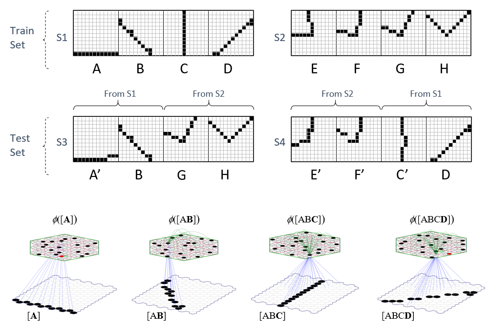
This section is currently just a stub. It will present results from my 2017 paper “A Radically New Theory of how the Brain Represents and Computes with Probabilities”, demonstrating fixed-time update of the likelihood distribution (and indirectly, the total probability distribution) over ALL items stored in a coding field. Moreover, these results concern learning and inference over spatiotemporal patterns, i.e., sequences, not simply spatial patterns as in the prior section. This entails a generalization of the CSA (compared to that described with respect to Fig. 7) in which the SDR chosen for the input at time t depends on both the bottom-up signals (the u values) and the signals arriving via the recurrent (a.k.a. “horizontal”) matrix (green arrows) from the code at time t-1. Note however, that the generalized CSA remains a fixed-time algorithm. The training set used in that paper consists of the two sequences, S1 and S2, shown in Fig. 8. The test sequence, S3, consisted of the first two items of S1 followed by the last two items of S2, the idea being that we “garden path” the model and see how well it can recover when it encounters the anomaly. Test sequence S4 was comprised of the first two items of S2 and the last two of S1. And, we also added some pixel-wise noise to some of the test sequence frames to make the inference problem harder. At bottom of Fig. 8, we show the model on the four items of training sequence S1, showing the bottom-up weights that were increased on each frame and a subset of the recurrent weights (green) that were increased. The full description of this result would make this already very long blog much longer and so will be done in a separate blog. For now. the reader can look at the 2017 paper to see the full description. As you will see, Sparsey, easily deals with these ambiguous moments of sequences, and rapidly recovers into the correct internal SDR chain as subsequent items of the sequence come in.

Figure 8: Learning Set of Two 4-Step Sequences

Further Remarks on Algorithmic Parallelism vs. Quantum Parallelism

As noted at the outset, with respect to an N-qubit quantum computer, quantum parallelism is usually described as the phenomenon in which the execution of a single physical, atomic operation simultaneously operates on all 2N basis states in the superposition. For example, applying a Hadamard transform on the N qubits results in a physical superposition in which all 2N basis states have equal probability amplitude, thus equal probability.  More generally, in an instance of the Deutsch-Jozsa algorithm, a circuit of quantum gates is designed that computes some function, f().  A single physical application (execution) of that circuit on the N-qubit system operates on all 2N basis states, φi, held in superposition, yielding a new superposition of the 2N values, f(φi). I make two key observations about this description of quantum parallelism.

  1. I emphasized “designed” above to highlight the fact that most of the work in quantum computing has not focused on learning.  Ideally, we want learning systems, and in particular, unsupervised learning systems, that realize/achieve quantum parallelism.  That is, what we ideally want is a computer that can observe a physical dynamical system of interest through time—e.g., multivariate time series of financial/economic data, or biosequence/medical data, video (frame sequences) of activities/events transpiring in spaces, e.g., airports, etc.—and learn the dynamics from scratch.  By “learn the dynamics”, I mean learn the “basis states” of the system and learn the likelihoods of transitions between states, all at the same time.
  2. In the above description of quantum parallelism, a single atomic physical operation is described as operating on, i.e., updating the probability amplitudes of, all 2N basis states held in the superposition in the N qubits.  However, if these basis states in fact represent the states of a natural physical system, then while it is true that there are formally 2N basis states, almost all of them will correspond to physical states that have near-zero probability of ever occurring. Moreover, almost all of the 2N x 2N state transitions will also have near-zero probability of occurring. That is, the strong hierarchical part-whole structure of natural entities and natural dynamics, e.g., operation of natural physical law, will, with probability close to 1, never bring the system into such states.  These states likely do not need to be explicitly represented in order for the model to do a good job emulating the system’s evolution through time, and thus, allowing good predictions.  Thus, if we take “almost all” seriously, then the number of basis states that, in practice, need to be represented (held) in superposition may be exponentially smaller than 2N, i.e., polynomial (and perhaps low-order polynomial) in N.

Sparsey addresses both these observations.  Regarding the first, Sparsey was developed from inception as a biologically plausible, neuromorphic model of learning [as well as of memory (both episodic and semantic), inference, and cognition] of spatiotemporal patterns (handling purely spatial patterns as a special case).  In that domain, the represented entities are sensory inputs, e.g., visual input patterns (preprocessed as seen here, here, or here), which are not known a priori, but have to be learned by experiencing the input domain, i.e., the “world”.14 In contrast, in quantum mechanics, the entities are the physical basis states themselves, which are defined a priori, in terms of the values of (generally, one or a few) fundamental physical properties, e.g., spin angular momentum, polarization, of the system’s atomic constituents.  Thus, quantum mechanics proper, has NOT been a theory about learning.  Not surprisingly, quantum computing has largely also NOT been about learning.  Most quantum computing algorithms in the literature, e.g., Shor’s, Grover’s, are fixed algorithms that perform specific computations.

Regarding the second observation, a Sparsey coding field15 has a large storage capacity, not exponential in the units, but large. Specifically, simulation results show faster than linear (i.e., as some low-order polynomial) capacity scaling in the units, and linear scaling in the weights.  N.b.: Those results from my 1996 Thesis research were done on a slightly different architecture.  While they apply with full force to the current architecture (see Fig. 2), I don’t want to introduce the older architecture in the main flow of this essay and so direct the reader to this page to see the detailed results.  Fig. 9 summarizes those results.  In these experiments, the coding field consisted of Q=100 WTA CMs, and the number of units per CM, K, was varied from 8 to 40 in steps of 4. Here, the relevant matrix was the recurrent matrix that fully connected the coding field units to themselves. Thus, the matrix for the largest model tested, whose coding field had 100×40=4000 units, had 16 million weights. The learning protocol was temporal Hebbian, i.e., all weights from units active at T to units active at T+1 were set to 1 (either increased from 0 to 1, or left at 1). Thus, the SDRs of successive items of a sequence were “chained” together (as in Fig. 6). Also, in these experiments, the input level was a 10×10 binary pixel array and the objective was to store as many as possible 10-frame-long sequences, where each frame had 20 active pixels, as shown in Fig. 9a. 

Figure 9: Storage Capacity of a Sparsey Coding Field.

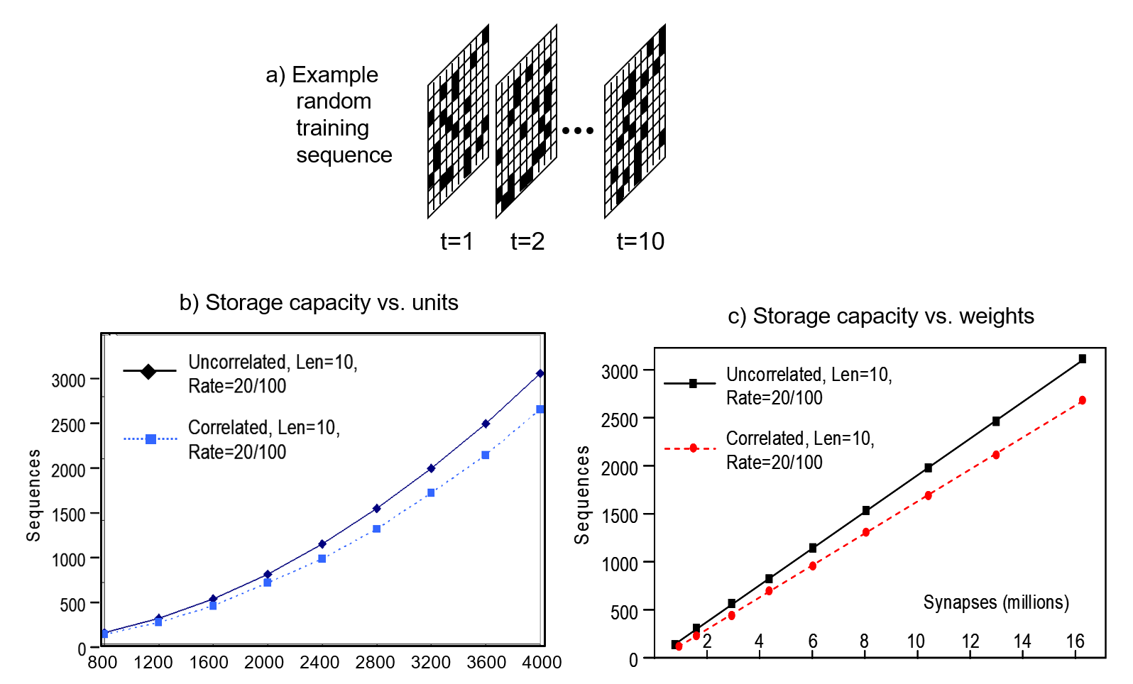
Two input conditions were tested.  In the first, labelled “uncorrelated”, all frames of all sequences were generated randomly.  In the second, labelled “correlated”, we first created a lexicon of 100 frames, that were also generated randomly.  The actual sequences of the correlated training set were then created by making 10 random draws (with replacement) from the lexicon.  This “correlated” condition was intended to model the linguistic environment, i.e., where the items of sequences occur numerous times and in numerous sequential contexts.  As Fig. 9b shows, the number of such sequences that can be safely stored, i.e., stored so that all sequences can be retrieved with accuracy above some threshold, here, ~97%, grows faster than linearly in the units.  Note that here, retrieval was tested by reinstating the code of the first item of a sequence and measuring how precisely the remaining nine items were read out, i.e., these were recall, not recognition, tests. So this is a lot of information being stored and recalled.  In the largest model tested (4000 units, 16 million wts), over 3,000 of these random 10-frame sequences were safely stored, despite being presented once each. Fig. 9c shows that the capacity scales linearly in the weights.

The classical realization of quantum entanglement

Quantum entanglement (QE) is the phenomenon in which two16 particles, X and Y, become perfectly correlated (or anti-correlated) with respect to some property, e.g., spin, even though neither particle’s value of that property is determined. In fact, the only definite physical change that can be said to occur at the moment of entanglement is that a dependence is introduced between X and Y such that if one is subsequently measured and found to have spin up, the other will instantly have spin down. X and Y are said to be in the “singlet” state: they are formally considered to be a single entity.17 At the moment of measurement, X and Y become unentangled, i.e., the singlet state, which is a superposition of the two basis states, collapses (decoheres) to one of the two possible basis states. This phenomenon occurs regardless of how far apart X and Y may be when either is measured, which implies superluminal propagation of effect (transfer of information), i.e., Einstein’s “spooky action at a distance”.

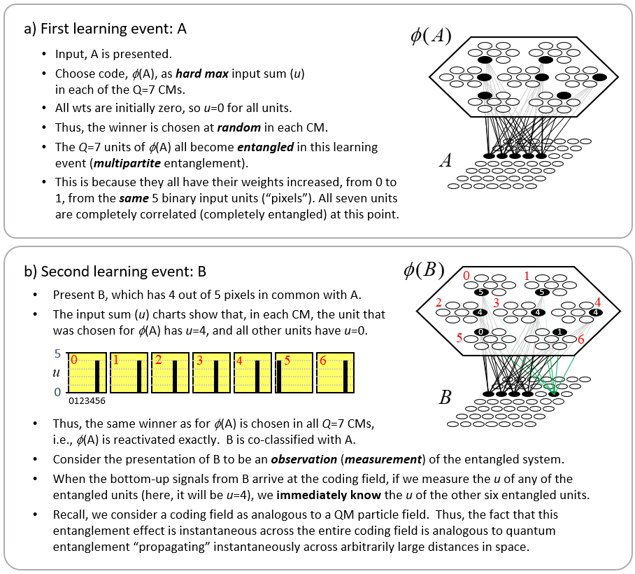
Is there another way of understanding the phenomenon of QE? Yes, I will provide a new, classical explanation of QE here, in terms of Sparsey’s SDR codes and the weight matrices that connect (including recurrently) coding fields. First, recall, in a side comment above, I proposed that a Sparsey coding field is the analog of a QM particle field, let’s say, the electron field. Thus, Sparsey’s binary units should be viewed as analogs of QM’s electrons.18 Fig. 10 illustrates the phenomenon of entanglement in Sparsey. Note however that this example uses a simpler code selection algorithm than Sparsey’s actual CSA, described above. Specifically, winners will now be chosen using hard max instead of soft max. Fig. 10a shows the learning event in which an input pattern, A (the five active binary units, “pixels”), has been presented. Note that all inputs will be constrained to have the same number of active pixels. The code (SDR), φ(A), is then chosen by picking the unit with the hard max input sum (u) in each CM. Since all weights are initially zero, all units have u=0, so the winners (black) are chosen randomly. Finally, the association from A to φ(A) is formed by increasing the depicted weights (black lines) from 0 to 1. The Q=7 units comprising φ(A) become entangled in this learning event.19 They become entangled because their individual afferent weight matrices are changed in exactly the same way: they all have their afferent weights from the same five active pixels increased from 0 to 1. Note also that at this point, these seven units are completely redundant (completely correlated).

To see why this learning event constitutes entanglement, consider the presentation of a second input, B, in Fig. 10b. B has 4 out of 5 pixels in common with A. Suppose we can observe (measure) any of φ(A)’s units, i.e., we have an “electrode” in it. Then, when the bottom-up signals arrive from the input level, as soon as we measure u for any one of those units, and find it to have u=4, we instantly know the other six units of φ(A) also have u=4. Just as in QM, where entanglement “propagates” across arbitrarily large distances of an actual quantum field, which spans all of space, this example shows that entanglement “propagates” across the full extent of of the coding field. But unlike the case for QM, we can directly see the physical mechanism underlying this “propagation”. In fact, it is clear that it is not propagation at all: no signal propagates across the coding field in this scenario. Again, it’s simply the correlated changes that occurred in the weight matrix that impinges the coding field during the learning, i.e., entanglement, event, which explains how we can instantly know the value of some variable (u) at arbitrarily remote distances from where a measurement takes place.

Figure 10: Entanglement in Sparsey

So, what is this telling us? It’s telling us that the weight matrix is analogous to a force-carrying (boson) field of QM. After all, it’s the boson fields through which effects (information) propagates through space and its the weight matrices of Sparsey (or of any neuromorphic model) through which effects/information propagate. I further emphasize that a boson field fills all of space (and is superposed with all other boson and fermion fields) and in particular, allows transmission of an effect from any point in space to any other (at ≤ speed of light). In other words, a boson field completely connects any particular fermion field. Likewise, we require that the matrix between any two Sparsey coding fields (including recurrently) and between a coding field and an input field also be complete. But of course there is at least one huge difference between a boson field and a weight matrix. The individual weights comprising a Sparsey weight matrix are changed by the signals that pass through them. In contrast, no such concept of learning, at least of permanent learning, applies to a boson field. I believe this is at the heart of why no one has have ever figured out a local “hidden variables” (HV) mechanism for QM. In all discussions I’ve seen, it seems that any such local HVs were posited to be located within the particles themselves. Recent experiments showing violation of Bell’s inequality refute those types of local HV explanations. But again, in Sparsey, as shown in Fig. 10, the physical changes underlying entanglement occur outside the entangled entities (the units) themselves; they occur in the weights. These weights still constitute local variables [after all, any individual weight is immediately local (adjacent) only to its source and destination units]20, but they are not hidden variables. I suspect that the recent Bell inequality violation findings do not refute the type of “local variables” explanation given here.

There is a great deal more to present regarding this new explanation of QE. I’ll do that in subsequent posts. For now, I just want to end this section by noting that this same principle/mechanism applies when thinking about how groups of neurons somehow become bound together to act as an integral code (single entity), i.e. how Hebbian “cell assemblies” form. Most prior computational neuroscience theories for cell assemblies, e.g., Buszaki’s “Synapsembles” (2010), propose that they form by virtue of changes made to weights directly between the member units of the cell assembly. But I have previously described how the “binding” mechanism described here–correlated changes to afferent and efferent weight matrices of the bound units–could easily explain the formation of cell assemblies in the brain’s cortex.

Summary

Coming soon…..

Representing Entities as Sets Provides a Classical Explanation of Quantum Entanglement

Entanglement is usually described in terms of a physical theory, namely quantum theory (QT), wherein the entities formally represented in the theory are physical entities, e.g., electrons, photons, composites (ensembles) of any size. In contrast, I will describe entanglement in the context of an information processing model in which the entities formally represented in the theory are items of information. Of course, any item of information, even a single bit, is ultimately physically reified somewhere, even if only in the physical brain of a theoretician imagining the item. So, we might expect the two descriptions of entanglement, one in terms of a physical theory and the other in terms of an information processing theory, to coalesce, to become equivalent, cf. Wheeler’s “It from Bit”. This essay works towards that goal.

The information processing model used here is based on representing items of information as sets, specifically, (relatively) small subsets, of binary representational units chosen from a much larger universal set of these units. This type of representation has been referred to as a sparse distributed representation (SDR) or sparse distributed code (SDC).21 We’ll use the term, SDC. Fig. 1 shows a small toy example of an SDC model. The universal set, or coding field (or memory), is organized as a set of Q=6 groups of K=7 binary units. These groups function in winner-take-all (WTA) fashion and we refer to them as competitive modules (CMs). The coding field is completely connected to an input field of binary units, organized as a 2D array (e.g., a primitive retina of binary pixels), in both directions, a forward matrix of binary connections (weights) and a reverse matrix of binary weights. All weights are initially zero. We impose the constraint that all inputs have the same number of active pixels, S=7.

Fig. 1: Small example of an SDC-based model. The coding field consists of Q=6 competitive modules (CMs), each consisting of K=7 binary units. The input field is a 2D array of binary units (pixels) and is completely connected in both directions, i.e., a forward and a reverse matrix of binary weights (grey lines, each on represents both the forward and the reverse weight).

The storage (learning) operation is as follows. When an input item, Ii, is presented (activated in the input field), a code, φ(Ii) consisting of Q units, one in each of the Q CMs, is chosen and activated and all forward and reverse weights between active input and active coding field units are set to one. In general, some of those weights may already be one due to prior learning. We will discuss the algorithm for choosing the codes during learning in a later section. For now, we can assume that codes are chosen at random. In general, any given coding, α, unit will be included in the codes of multiple inputs. For each new input in whose code α is included, if that input includes units (pixels) that were not active in any of the prior inputs in whose codes α was included, the weights from those pixels to α will be increased. Thus, the set of input units having a connection with weight one onto α can only increase with time (with further inputs). We call that set of input units with w=1 onto α, α’s tuning function (TF),

The retrieval operation is as follows. An input, i.e., a retrieval cue, is presented, which causes signals to travel to the coding field via the forward matrix, whereupon the coding field units compute their input summations and the unit with the max sum in each CM is chosen winner, ties broken at random. Once this “retrieved” code is activated, it sends signals via the reverse matrix, whereupon, the input units compute their input summations and are activated (or possibly deactivated) depending on whether a threshold is exceeded. In this way, partial input cues, i.e., with less than S active units, can be “filled in” and novel cues that are similar enough to previously (learned) inputs can cause the codes of such, closest-matching learned inputs to activate, which can then cause (via the reverse signals) activation of that closest-matching learned input.

With the above description of the model’s storage and retrieval operations in mind, I will now describe the analog of quantum entanglement in this classical model. Fig. 2 shows the event of storing the first item of information, I1, into this model. I1 consists of the S=7 light green input units. The Q=6 green coding field units are chosen randomly to be I1‘s code, φ(I1), and the black lines show some of the weights that would be increased, from 0 to 1, in this learning event. Each line represents both the forward and reverse weight connecting the two units. More specifically, the black lines show all the forward/reverse weights that would be increased for two of φ(I1)’s units, denoted α and β. Note that immediately following this learning event (the storage of I1), α and β have exactly the same TF. In fact, all six units comprising φ(I1) have exactly the same TF. In the information processing realm, and more pointedly in neural models, we would describe these six units as being completely correlated. That is, all possible next inputs to the model, a repeat presentation of I1 or any other possible input, would cause exactly the same input summation to occur in all six units, and thus, exactly the same response by all six units. In other words, all six units carry exactly the same information, i.e., are completely redundant.22

Fig. 2: The first input to the model, I1, consisting of the S=7 light green units, has been presented and a code, φ(I1), consisting of Q=6 units (green), has been chosen at random. All forward and reverse weights between active input and coding fields units are set to one. The black lines show all such weights involving coding units α and β.

As the reader may already have anticipated, I will claim that these six units are completely entangled.23 We can consider the act of assigning the six units as the code, φ(I1), as analogous to an event in which a particle decays, giving rise, for example, to two completely entangled photons. In the moment when the two particles are born out of the vacuum, they are completely entangled and likewise, in the moment when the code, φ(I1), is formed, the six units comprising it are completely entangled. However, in the information processing model described here, the mechanism that explains the entanglement, i.e., the correlation, is perfectly clear: it’s the correlated increases to the forward/reverse weights to/from the six units that entangles those units. Note in particular, that there are no direct physical connections between coding field units in different CMs. This is crucial: it highlights the fact that in this explanation of entanglement, the hidden variables are external, i.e., non-local, to the units that are entangled. The hidden variables ARE the connections (weights). This hints at the possibility that the explanation of entanglement herein comports with Bell’s theorem. The 2015 results proving Bell’s theorem, explicitly rule out only local hidden variables explanations of entanglement. Fig. 3 shows the broad correspondence between the information theory and the physical theory proposed here.

Fig. 3: Broad correspondence between the information processing theory described here (and previously throughout my work) and the proposed physical theory. This figure will generalized in a later section to include the recurrent matrix that connects the coding field to itself (and is also part of the bosonic representation), which is needed to explain how the physical state represented by the coding field is updated through time, i.e. the dynamics.

Suppose we now activate just one of the seven input units comprising I1, say δ. Then φ(I1) will activate in its entirety (i.e., all Q=6 of its units) due to the “max sum” rule stated above, and then the remaining six input units comprising I1 will be activated based on the inputs via the reverse matrix. Suppose we consider the activation of δ to be analogous to making a measurement or observation. In this interpretation, the act of measuring at one locale of the input field, at δ, immediately determines the state of the entire coding field and subsequently (via the reverse projection) the entire state of the input field [or more properly, input/output (“I/O”) field], in particular, the state of the spatially distant I/O unit, λ. Note that there is no direct connection between δ and λ. The causal and deterministic signaling went, in one hop, via the connections of the forward and reverse matrices. Thus, while our hidden variables, the connections, are strictly external (non-local) to the units being entangled (i.e., the connections are not inside any of the units, either coding units or I/O units), they themselves are local in the sense of being immediately adjacent to the entangled units. Thus, this explanation meets the criteria for local realism. This highlights an essential assumption of my overall explanation of quantum entanglement. It requires that physical space, or rather the underlying physical substrate from which our apparent 3D space and all the things in it emerge24, be composed of smallest functional units that are completely connected. In another essay, I call these smallest functional, or atomic functional, units, “corpuscles”. Specifically, a corpuscle is comprised of a coding field similar to, but vastly larger than (e.g., Q=106, K=1015), those depicted here and: a) a recurrent matrix of weights that completely connects the coding field to itself; and b) matrices that completely connect the coding field to the coding fields in all immediately neighboring corpuscles. In particular, the recurrent matrix allows the state of the coding field at T to influence, in one signal-propagation step, the state of the coding field at T+1. Thus, to be clear, the explanation of entanglement given here applies within any given corpuscle. It allows instantaneous, i.e., faster than light, transmission of effects throughout the region of (emergent) space corresponding to the corpuscle, which I’ve proposed elsewhere to be perhaps 1015 Planck lengths in diameter. If we define the time, in Planck times, that it takes for the corpuscle to update its state to equal the diameter of corpuscle, in Planck lengths, then signals (effects) are limited to propagating across larger expanses, i.e., from one corpuscle to the next, no faster than light.

Here I must pause to clarify the analogy. In the typical description of entanglement within the context of the standard model (SM), it is (typically) the fundamental particles of the SM, e.g., electrons, photons, which become entangled. In the explanation described here, it is the individual coding units that become entangled. But I do not propose that that these coding field units are analogous to individual fundamental particles of the standard model (SM). Rather, I propose that the fundamental particles of the SM correspond to sets of coding field units, in particular, to sets of size smaller than a full code, i.e., smaller than Q. That is, the entire state of region of space emerging from a single corpuscle is a set of Q active coding units. But a subset of those Q units might be associated with any particular entity (particle) present in that region at any given time. For example, a particular set of coding units, say of size Q/10, might always be active whenever an electron is present in the region, i.e., that “sub-code” appears as a subset in all full codes (of size, Q) in which an electron is present. Thus, rather than saying that, in the theory described here, individual coding units become entangled, we can slightly modify it to say that subsets of coding units become entangled.25

Returning to the main thread, Fig. 4 now describes how patterns of entanglement generally change over time. Fig. 4a is a repeat of Fig. 2, showing the model after the first item, I1, is stored. Fig. 4b shows a possible next input, I2, also consisting of S=7 active I/O units, one of which, δ is common to I1. Black lines depict the connections whose weights are increased in this event. The dotted line is to indicate that the weights between α and δ will have been increased when I1 was presented. Fig. 4c shows α’s TF after I2 was presented. It now includes the 13 I/O units in the union of the two input patterns, {I1 ∪ I2}. In particular, note that coding units, α and β are no longer completely correlated, i.e., their TFs are no longer identical, which means that we could find new inputs that elicit different responses in α and β. In general, the different responses, can lead, via reverse signals, to different patterns of activation in the I/O field, i.e., different values of observables. In other words, they are no longer completely entangled. This is analogous to two particles which arise completely entangled from a single event, going off and having different histories of interactions with the world. With each new interaction that either one has, they become less entangled. However, note that even though α and β are no longer 100% correlated, we can still predict either’s state of activation based on the other’s at better-than-chance accuracy, due to the common units in their TFs and to the corresponding correlated changes to their weights.

Fig. 4: (a) Repeat of Fig. 2 for reference. (b) Presentation of the second input, I2, its randomly selected code, φ(I2), and the new learning involving coding unit α. The weights to/from I/O unit δ are dashed since they were already increased to one when I1 was presented, i.e., δ was active in both inputs. (c) α’s TF is the union of all I/O units that are active in any input in whose code α was included. In particular, α and β are no longer completely entangled (correlated), due to this additional interaction α has had with the world.

Fig. 5 now shows a more extensive example illustrating the further evolution of the same process shown in Fig. 4. In Fig. 5, we show coding unit α participating in a further code, φ(I3), for input I3. And we show coding unit β participating in the codes of two other inputs, I4 and I5, after participating, along with α, in the code of the first input, I1. Panel d shows the final TF for α after being used in codes of three inputs, I1, I2 and I3. Panel g shows the final TF for β after being used in the codes for I1, I4 and I5. One can clearly see how the TFs gradually diverge due to their diverging histories of usage (i.e., interaction with the world). This corresponds to α and β becoming progressively less entangled with successive usages (interactions).

Fig. 5: Depiction of the continued diminution of the entanglement of α and β as they participate in different histories of inputs. Panel d shows the final TF for α after being used in codes of three inputs, I1, I2 and I3. Panel g shows the final TF for β after being used in the codes for I1, I4 and I5.

To quantify the decrease in entanglement precisely, we need to do a lot of counting. Fig. 6 shows the idea. Figs. 6a and 6b repeat Figs. 5d and 5g, showing the TFs of α and β. Figs. 6c and 6d show the intersection of those two TFs. The colored dots indicate the input from which the particular I/O unit (pixel) was accrued into the TF. In order for any future input [including any repeat of any of the learned (stored) ones] to affect α and β differently (i.e., to cause α and β to have different input sums, and thus, to have different chances of winning in their respective CMs, and thus, to ultimately cause activation of different full codes), that code must include at least one I/O unit that is in either TF but not in the intersection of the TFs. Again, all inputs are constrained to be of size S=7. Thus, after presenting any input, we can count the number of such codes that meet that criterion. Over long histories, i.e., for large sets of inputs, that number will grow with each successive input.

Fig. 6: (a,b) Repeats of Figs. 5d and 5g showing the TFs of α and β. (c,d) The union of the two TFs (black cells). The colored dots tell from which input the I/O unit (pixel) was accrued into the relevant coding unit’s TF.

A storage (learning) algorithm that preserves similarity

In the examples above, the codes were chosen randomly. While we can and did provide an explanation of entanglement under that assumption, a much more powerful and sweeping physical theory emerges if we can provide a tractable mechanism (algorithm) for choosing codes in a way that statistically preserves similarity, i.e., maps similar inputs to similar codes. In this section, I will describe that algorithm. The final section will then revisit entanglement, providing further elaboration.

A Simple explanation of the Holographic Principle

The holographic principle says that the maximum amount of information that can be contained in a volume (bulk) equals the amount of information that can be contained on the surface of that bulk. On first thought, this seems absurd: Common sense tells us that there is so much more matter comprising a bulk than comprising its surface. Yet, this is what the work of ‘t Hooft and others tells us. Fig. 1 (from ‘t Hooft’s 2000 paper, “The Holographic Principle”) shows a tiling in which each patch, of area equal to 4 x Planck area (~4 x 10-70 sq. m.), can hold one bit of information. Since black holes are the most dense objects, we can take this number, the area of the surface of a spherical volume in units of Planck areas divided by 4 to be an upper bound on the number of bits that can be stored in that volume. In fact, the explanation given in this essay suggests the upper bound is just slightly less than the area in Planck units.

Fig. 1: Linked from Gerard ‘t Hooft’s “The Holographic Principle” (2000). Depiction of the result that the number of bits of information contained in a black hole equals the area of the black hole’s surface in Planck areas divided by 4.

If the Planck length is the smallest unit of spatial size, then 2D surfaces in space have areas that are discretely valued and 3D regions have volumes that are discretely valued. Since the cube is the the only regular and space-filling polyhedron for 3D space, we therefore assume that space is a cubic tiling of Planck volumes as in Fig. 2. If the Planck volume is the smallest possible volume then it can have no internal structure. Thus, the simplest possible assumption is that it is binary-valued; either something exists in that volume (“1”) or not (“0”). I call these Planck-size volumes, “Planckons”. However, note that despite the ending “ons”, these are not particles like those of the Standard Model (SM). In particular, they do not move: they are the units of space itself.

Fig. 2: Space is a 3D tiling of Planck-size cubes. The “Planckons” are binary-valued.

I contend that that the this assumption, that space is a 3D tiling of binary-valued Planck cubes already explains the why the amount of information that can be contained in a volume is upper-bounded by the amount of information that can be contained on its surface, i.e., the holographic principle. For example, consider a cube-shaped volume of space, i.e., a bulk, that is 8 Planck lengths on each side, as shown in Fig. 3 (rose colored Planckons). This bulk, consists of 83 = 512 Planckons. Consider the layer of Planckons that forms the immediate boundary of this bulk. We can take the boundary to be just the union of the six 2D arrays of Planckons that are immediately adjacent to the six faces. Thus the boundary consists of 6 x 82 = 384 Planckons. In the case of a black hole, this boundary is the event horizon. The reason why we ignore the Planckons that run along just outside the edges of the bulk and those at the corners just outside the bulk is that we assume that physical effects can only transmit through faces of Planckons.26. The boundary constitutes a channel through which all physical effects, i.e., communication (information), to and from this bulk must pass. The number of unique states that the bulk can be in is 2512. On first glance, this suggests, that the amount of information that can be stored in this bulk is log22512bits, i.e., 512 bits. The number of unique states of the channel is only 2384, suggesting it can hold only log22384 = 384, bits of information. In fact, the holographic principle says that the number of bits storable in the channel is only 384 / 4 = 96 bits. However, the explanation developed here suggests the limit is just less than 384. The reason it’s not exactly equal to to 384 is a slight diminution due to edge and corner effects. In any case, the overall argument explains why the information storage capacity is determined by the area of the surface bounding a volume and not by the volume.

Fig.3: Depiction of a 3D bulk consisting of 8x8x8=512 binary Planckons and its boundary that is the union of the six 8×8 2D arrays of Planckons, for a total of 384 Planckons, that wraps the bulk.

Try to imagine possible mechanisms by which the states of Planckons submerged in the bulk could be accessed, i.e., read or written. Any such infrastructure and mechanism for implementing such read or write operations would have to reside in the bulk. E.g., perhaps one might imagine some internal system of say, 1-Planckon thick, buses threading through the bulk, providing access to those submerged Planckons. Thus, some of the 512 bulk Planckons cannot be available for storing information. While this would reduce the information storage limit to something less than the full volume in Planck volumes, it does not explain why it should be reduced all the way down to being approximately equal the number of Planckons comprising the 2D boundary.

Rather than address the 3D case directly, let’s reduce the dimension of the problem by one. Accordingly, Fig. 4 shows a 2D space, a 2D bulk, the 5×5 array of rose Planckons, wrapped by a 1D boundary, comprised of 20 white Planckons.27 The analogy of the 3D version of the holographic principle would predict that the amount of information that can be stored in the 25 Planckon (25 bit) bulk equals the amount of information that can be stored in the 20 Planckon boundary, again, disregarding the divisor of four.

Fig. 4: (a,b) a 2D bulk (red square) consisting of 5×5 Planckons, surrounded by a 1D boundary of Planckons. (c) The 16 light blue Planckons of the bulk are in direct contact with the boundary. Assuming that physical (causal) effects, i.e., signals, can only be transmitted through shared edges, not corners, then only these 16 bulk Planckons can be written or read from (through) the boundary.

Since we assume that physical effects can only be transmitted through edge connections (not corners), only the 16 bulk Planckons comprising the outermost, one-Planckon-thick shell of the bulk (blue Planckons) are directly accessible from the boundary (arrows show examples of access paths). We can imagine those 16 bulk Planckons, as a memory of bits just as in a regular computer memory and the Planckons comprising the boundary (perhaps along with additional Planckons extending into the space beyond the boundary) to be a bus, or connection matrix, for accessing (writing or reading) these 16 bits. In any case, the innermost nine Planckons of the bulk (rose Planckons in Fig. 4c) are not directly accessible from the boundary. We then have the question as to how the states of those innermost nine bulk Planckons could help to increase the storage capacity of the bulk.

Rather than attempt to construct such an infrastructure and (read and write) operations, let’s instead imagine how submerged Planckons might be able to be seen through other Planckons, and thus possibly affect the state of the (one or more) boundary Planckons. We can actually make the problem easier, and without loss of generality, by reducing the problem by one dimension.

The answer is that they cannot increase the storage capacity. Why?

It seems there are two approaches

  • We can treat the bulk as a cellular automata in which case we define a rule by which a Planckon updates its states as a function of its own state and those of its four edge-adjacent neighbors. In this case, there is only one rule, which operates in every Planckon. In particular, this means all Planckons are of the same type.
  • We can treat consider the bulk’s Planckons as being of two types: a) ones that hold a binary state, i.e., bits of memory, as we have already postulated for the outermost 16 Planckons of the bulk; and b) ones that implement communication, i.e., transmit signals, in which case, we’re allowing that the communication infrastructure (bus, matrix) now extends into the bulk itself.

In the first approach, for there to be a positive answer to the challenge question, there must be an update rule (i.e. dynamics) which allows 25 bits to be stored and retrieved. In the second approach, where we partition the bulk’s Planckons into two disjoint subsets, those that hold state, which we will call a memory, or a coding field, and those that transmit signals, we need to define the structure (topology) of both parts, the coding field and the signal transmission partition.

…STILL BEING WRITTEN…

So it seems that we are led to the concept of a corpuscle of space. As defined elsewhere, the corpuscle is the smallest completely connected region of space, i.e., where the coding field Planckons are completely connected to themselves (a recurrent connection) and completely connected to the Planckons comprising the corpuscle’s boundary. So in this case, the model is explicitly not a cellular automata, where the physical units tiling a space are connected only to nearest neighbors according to the dimension of the space in which the physical units exist. Rather, by assigning some Planckons to be for communication and some for states, we make possible connectivity schemes that are not limited to the underlying space’s dimension, but rather can allow arbitrarily higher dimensionality (topology) for subset of Planckons devoted to representing state.

So it’s just as simple as that. If space is discrete, then the amount of information that can be contained in a 3D volume equals the amount of information that can be contained in its 2D (though actually, one-Planckon thick) boundary. Also, note that the argument remains qualitatively the same if we consider the bulk and boundaries as spheres instead.

There are only 2384 possible messages (signals) we could receive from this bulk. So even though there are vastly more , i.e., 2512, unique states of the bulk, all of those states necessarily fall into only 2384 equivalence classes. And similarly, there are only 2384 messages we could send into the bulk, meaning that all possible states of the vastly larger world outside the bulk similarly fall into only 2384 equivalence classes. No matter what computational process we can imagine that operates inside the bulk, i.e., no matter which of it’s 2384 states is produced by such process, and furthermore, no matter how many steps the process producing that state takes, it can only produce 2384 output messages.

A well-known quantum computation theorist told me that the above is simply a re-statement of the holographic principle, not an explanation. In particular, he said that I need to explain why we could not send more than 384, or in fact, all 512 bits of information into the bulk by sending multiple messages. So here is the explanation of why multiple messages doesn’t help.

A Physical Theory based on Sets, Not Vectors: Part 1

In quantum theory (QT), physical states are formally represented as vectors (in Hilbert space). As we all know, a vector is equivalent to a point, which is 0-dimensional, and therefore has zero extension. This suggests that any physical state, and thus any physical particle that is part of the ensemble present in that state, formally has zero extension. However, quantum theory avoids this interpretation by making the Hilbert space dimensions themselves, i.e., its basis vectors, be functions of space, not simply scalar-valued. Specifically, the value of any particular dimension is the absolute value of a wave function, i.e., of a particular probability density function over space. This is the mechanism by which quantum theory imparts spatial extent to physical entities. And it is central in facilitating the assertions by some quantum theorists that a purely formal mathematical object, i.e., a probability density function, used to represent a physical object is more real than the physical object itself. It’s also the underlying reason why in QT, all states that can exist actually do simultaneously exist, and furthermore, simultaneously exist at all instants of time. Somehow, they all occupy the same physical space, i.e., they all exist in physical superposition, and they do so for all of time. Make no mistake: quantum theory says that at every moment of time, all possible physical states exist in their entireties: in particular, QT does NOT say that any particular state partially exists. Rather, it says that the probability of actually observing any state, all of which fully physically exist, is what varies.

The choice to represent states as vectors can perhaps be considered the most fundamental assumption of QT. It implies that the space in which things arise and events occur exists prior to any of those things or events. This seems a perfectly reasonable, even unassailable assumption: indeed, how could it be otherwise? How can anything exist or anything happen unless there is first a space (and a time) to contain them? But that assumption is assailable. In fact, there is a simple formalism that completely averts the need for a prior space to exist. That formalism is sets. We can build dimensions, and therefore a space, out of sets. Specifically, a formal representation of dimension can be built out of, or emerge from, a pattern of intersections amongst sets, specifically amongst subsets chosen from a universe of elements, as explained in Fig. 1.

At top of Fig. 1, we show a universe of 18 binary elements. These elements happen to be arranged in a line, i.e., in one dimension. However, we’ll be treating the elements as a set: thus, their relative positions (topology) doesn’t matter; only the fact that they are individuals matters. Fig 1 then shows three subsets that represent, or are the codes of, three states, A-C, of this tiny universe, e.g., state A is represented by the set (code), {1,4,7,10,12,15}, etc. Thus, we will also refer to this universe as a coding field (CF). We assume that the codes of all states of this universe are subsets of the same fixed size, Q=6. The bottom portion of Fig. 1 shows the pattern of intersection of the three states with respect to state A. This pattern of intersection sizes imposes a scalar ordering on the states, i.e., a dimension on which the states vary. If we wanted, we could name this dimension, “similarity to A”. The pattern of intersections carries the meaning, “B is more similar to A than C is”. Thus, set intersection size serves as a similarity metric. No external coordinate system, i.e., no space, is needed to represent the ordering (more generally, similarity relation) over the states. The dimension is emergent. My 2019 essay, “Learned Multidimensional Indexes“, generalizes this to multiple dimensions.

Figure 1: Explanation of how a spatial dimension can emerge as a pattern of intersections over sets.

To be clear, my proposed set-based theory of physical reality does require the prior existence of something, but that something is not a (vector) space, but rather a set, i.e., a universal set. Specifically, I propose that the set of all physical units comprising the universe is the set of Planck-length (10-35 m) volumes that tile the physical universe, as in Fig. 2 (left). So let’s call these quanta of space, planckons. N.b.: Figs. 2 thru 4 depict the set of planckons as tiling a 3-space, i.e., as “voxels”. However, the 3D topology is not used in the proposed model’s dynamics: the rule for how the state evolves does not use the relative spatial information of the planckons. As described herein, the apparent three spatial dimensions of the the universe, and any other observables, emerge as patterns of intersection over sets chosen from that underlying set of planckons, and as temporal patterns of evolution of those patterns (e.g., to explain movement through apparent macroscopic spatial dimensions). So to emphasize, Planckons do not move. Furthermore, the set of all planckons is partitioned into two sets, one being the underlying physical reification of matter, the fermionic planckons, or “flanckons“, and one being the underlying physical reification of forces (i.e., of transmission of effects, i.e., of signals), the bosonic planckons, or “blanckons“. The two partitions are intercalated at a fine scale, many orders of magnitude below that probed by experiment thus far (described shortly). And furthermore, planckons are binary-valued: at any time T, a planckon is either “active” (“1”) or “inactive” (“0”). For the case of blanckons, “active/inactive” can be viewed as representing the weight of a connection, 1 or 0, as in a binary weight matrix. I propose that in any local region of space (defined below), the matter and force content at T is present as a sparse subset of the flanckons being active, as suggested in Fig. 2 (right), though this picture is refined in Figs. 3 and 4. In fact, the proposed sparseness is many orders of magnitude greater than Fig. 2 (right) suggests.

Figure 2: (left) Space as a 3D tiling of Planck-scale “voxels”, or quanta of space, called planckons. (right) The planckons are binary-valued and partitioned into fermionic and bosonic subsets (that partitioning is not depicted here). At any time T, a subset of the planckons in a local volume (described below) either exists (is active) or does not exist (is not active).

Before continuing with the set-based physical theory, let me say that it was first, and still is foremost, a theory of how information is represented and processed in the brain (specifically in cortex). I am a computational neuroscientist, not a physicist, and the key insight underlying that theory, called Sparsey, is that all items of information (informational entities) represented in the brain are represented as sets, specifically sparse sets, of neurons (formalized as having binary activation), chosen from the much larger population (field) of neurons comprising a local region of cortex.28 Sparsey and the analogy between it and the set-based physical theory was described in some detail in my earlier essay, “The Classical Realization of Quantum Parallelism”. The explanations of superposition and of entanglement given in that earlier essay and which will be improved in part 2 of this essay come as direct, close analogs from the information-processing theory. In fact, the only difference between the two theories is that in the information-processing version, the elements comprising the underlying set from which the codes of entities (i.e., percepts, concepts, memories), and of spatial/temporal relationships between entities (i.e., part-whole, causal, etc.) are drawn are taken to be bits (as in a classical computer memory), whereas, in the physical theory, the elements comprising the underlying set are “its“, or as we’ve already called them, planckons, cf. Wheeler’s “It from Bit” (discussed here).

In focusing now on the physical theory, the first order of business is to refine Fig. 2, in particular, to define a local region of space, which is the fundamental functional unit of space, called a “corpuscle“, and describe how it consists of a fermionic and a bosonic partitions. By fundamental functional unit of space, I specifically mean the largest completely connected volume of space, which will be explained in the next few paragraphs. Fig. 3 (right) shows a “corpuscle“, which, for concreteness, we can assume to be a cube, 1015 Planck lengths, or roughly, 10-20m, on a side, thus far smaller than the smallest distance directly measured experimentally thus far (10-18m). It consists of two partitions:

  1. Flanckon partition: representing the fermionic, i.e., matter, state of the corpuscle; and
  2. Blanckon partition: representing the transitions from one matter state of the corpuscle to the next or to the next state of a neighboring corpuscle. Thus, this partition represents the bosonic aspect of reality, i.e., transmission of effect, or operation of forces.

The flanckon partition is far smaller, i.e., consists of far fewer planckons, than the blanckon partition and it is embedded (intercalated) sparsely and homogeneously throughout the corpuscle, i.e., throughout the far larger blanckon partition. Fig. 3 (left) shows the corpuscle’s flanckon partition “pulled out” from corpuscle, revealing its sub-structure, namely that it consists of Q winner-take-all (WTA) competitive modules (“CMs“) (shaded rose), each comprised of K flanckons. N.B.: While the CMs are depicted as being only 5 Planck lengths on each side in this figure, we assume they are far larger, e.g., 105 Planck lengths on each side, thus containing 1015 flanckons. These CMs are dispersed sparsely and homogeneously throughout the corpuscle’s far larger number of blanckons (white) as shown in Fig. 3 (right).29 The matter state of the corpuscle is defined as a set of Q active flanckons (black), one in each of the corpuscle’s Q CMs. N.B.: The fact that the CMs act as WTA modules, where exactly one of its flanckons can be active (“1”) at any time, T, is an axiom of the theory. Also note that in the figures, CMs without a black flanckon can be assumed to have one active flanckon at some internal position.

Figure 3: (right) The “corpuscle”, the fundamental functional unit of space. (left) Depiction the flanckon partition of the corpuscle, which consists of a set of Q winner-take-all (WTA) competitive modules (CMs) (rose), each comprised of K flanckons. The CMs are dispersed sparsely and homogeneously throughout the corpuscle’s far larger number of blanckons (white cubes). Note that while in this figure, the CMs are depicted as 5x5x5, as noted below, we assume they are in fact much larger, i.e., 105x105x105, and that the corpuscle is 1015x1015x1015.

As stated above, the blanckon partition provides the means by which effects (signals, forces) can be transmitted from a corpuscle’s matter state at T, both recurrently to its own state at T+1, as well as to the six neighboring, face-connected corpuscles (the universe is hypothesized to be a cubic tiling of corpuscles as shown in Fig. 4) at T+1. Given that the matter state of every corpuscle is a sparse activation pattern over a set of N = Q x K flanckons (again, which are binary valued), in order to instantiate any possible transition, i.e., mapping, from the matter state of a corpuscle at T, either recurrently to itself or to a neighboring corpuscle, at T+1, we require the corpuscle’s flanckon partition to be completely connected to itself and to its neighbors. Thus, if the corpuscle contains N flanckons, then it must contain at least 7 x N2 blanckons, a matrix of N2 blanckons for the recurrent matrix to itself, and a matrix of N2 blanckons connecting to the flanckons in each its six face-connected neighboring corpuscles. So this is what I meant above by the corpuscle being “the largest completely connected volume of space”: it is the largest volume of space for which dynamics, i.e., transitions from one state to the next, in both that volume and its neighbors can be a total function (of the prior state).30 In particular, no volume consisting of two of more corpuscles can be completely connected. Being the largest volume of space for which the time evolution of state is a total function, the corpuscle is the natural scale for defining the states and dynamics of universe, justifying referring to the corpuscle as the fundamental functional unit of space.

Fig. 4. Space as a 3D cubic tiling of corpuscles., each comprised of a flanckon partition [a set of CMs (rose), only some of which are visible as most will beneath the corpuscle’s faces], and a blanckon partition [all the other Planckons (white) of the corpuscle]. As described earlier, each corpuscle is a functional unit of space: a) whose matter state at time T is specified by the set of active flanckons (black), one per CM (the active flanckon does not appear in many CMs because it is not at a visible surface of the CM); and b) whose state at T+1 is determined by the signals arriving via the blanckons, both from its own active flanckons at T and from flanckons active at T in each of its six face-connected neighboring corpuscles.

The space of possible matter states of this fundamental region of space is the number of unique sets of active flanckons in the corpuscle, which is KQ (again, flanckon partition is organized as Q CMs, each with K flanckons, exactly one of which is active at any T). For example, if Q = 106 and K = 1015 (because we assumed above that the CMs are actually 105 Planck lengths on each side), then the number of unique matter states specifiable for the corpuscle, which again, is a cube of space only 10-20m on a side, is 1015,000,000. The transitions between states of a single corpuscle are specified in the binary pattern over that corpuscle’s recurrent blanckon matrix. This pattern of binary weights of the corpuscle’s recurrent blanckon matrix instantiates the operation of physical law, i.e., the dynamics (of all forces), for the individual corpuscle, which, again, is the fundamental functional unit of space. The weight pattern of this recurrent blanckon matrix in conjunction with those of the other six blanckon matrices (one to each of the six neighboring corpuscles), fully specifies the operation of physical law at all scales throughout the universe. That is, all effects are local: there is no action at a distance. Note: While the pattern over a corpuscle’s flanckon partition, i.e., its matter state, will generally change from one moment to the next, the pattern over the blanckons, again, which instantiates physical law, is fixed through time.

What do we mean by “instantiate physical law”. In the first place, we mean that the state transitions determined by the blanckon matrix are consistent with macroscopic observations, e.g., that a state at time T, in which a body is moving with speed s in some direction, will transition to a state at T+1, in which that body is at a new location along the line of motion and determined by s. The larger is s, the further the body is in the state at T+1. In other words, the transitions must exhibit the the kind of smoothness, or spatiotemporal continuity, that characterizes macroscopic physical law, not just for inertial movement, but for the macroscopic manifestations of all physical forces.31 Yet another way of stating this criterion is that the transitions must bring similar initial states into similar successor states, or in yet other terms, that the blanckon partition (which is a effectively a set of seven completely connected binary weight matrices, a recurrent one and six bipartite ones connecting to the six adjacent corpuscles) must preserve similarity. As explained with respect to Fig. 1, since states are represented as (extremely sparse) sets, the natural measure of similarity is intersection size.

Given that each of the possible matter states of a corpuscle is represented by a set and that more similar states will be represented by more highly intersecting sets, the essential question for the theory becomes:

  • Is the set of corpuscle states needed to explain all observed (i.e., possible) physical phenomena small enough so that the corpuscle’s blanckon matrix can produce all state transitions subsumed in the set of all possible physical phenomena?

That is, two similar states, S1 and S2, will have many of their flanckons in common. Since the blanckon partition (binary weight matrix) is permanently fixed, whenever either state occurs, that common set will send the same signals via the blanckon partition. While the non-intersecting portion of either state will send different signals via the blanckon partition in any such instance, we must specify a disambiguating mechanism by which the correct successor state reliably, in fact deterministically, occurs in both instances, i.e., despite the “crosstalk” interference imposed by the set of flanckons common to S1 and S2. Such a disambiguating mechanism was first explained in the context of the information-processing version of this theory, Sparsey, in my 1996 thesis, and many times since, and need not be described here again in detail. The reader can refer to those earlier works for the detailed explanation. The thesis in particular, showed that a large number of state transitions can be embedded in a single, fixed binary matrix. We now develop insight suggesting that for a volume of space as small as we hypothesize for the corpuscle, i.e., 10-20m on a side, the number of possible physical states needed to explain all higher-level phenomena might not be that large. The vast richness of variation observed at macroscopic scales might plausibly be produced by a relatively small canonical set of states, and a correspondingly small set of transitions, at the fundamental functional scale, i.e., the corpuscle scale, of the universe. Of course, stated this generally, such distillation is the goal of all science, especially physics, both classical and quantum. However, it is the dynamics in particular, i.e., the rules for how state changes, that is explicitly reduced to a small number in the edifice of science thus far. The range of states to which the the small number of rules can be applied has always been conceptualized as essentially infinite. In stark contrast, the claim here is that the underlying number of fundamental (matter) states is in fact discrete and relatively small. And the number of rules, i.e., of fundamental transitions is also discrete and relatively small, though substantially larger than in mainstream approach of science thus far.

So, on to discussing the plausibility of the assertion that only a relatively small number of fundamental matter states are needed for the corpuscle. At the outset, we acknowledge that the range of physical phenomena at the macroscopic scale appears vastly rich, and has historically been considered to vary continuously on any macroscopic dimension. However, we have no direct experience of the possible range of variation or of the granularity of variation at the scale of the corpuscle, 10-20m. Thus, from a scientific point of view, the number of fundamental matter states needed at the corpuscle scale (in order to account for all higher-level physical phenomena) is an open question. After all, the corpuscle is smaller than any distance ever measured (observed) thus far. In fact, while the fundamental particles of the Standard Model (SM), are generally treated as point masses, and thus being of zero size (again, the equivalence of vectors and points), the composite particles, in terms of which numerous experimental phenomena are described are assigned sizes far larger than the corpuscle. For example, a proton is estimated to be 10-15m in diameter, five orders of magnitude larger than the corpuscle, and the “classical radius of the electron” is also 10-15m (see here). Thus an individual proton (or electron) spans a diameter of 105 corpuscles. While it is possible that SM-scale particles can physically overlap, we will assume that at the scale of the corpuscle, they cannot.32 Thus, we assume that the number of unique particles that can be present in the corpuscle is the number of fundamental particles in the SM, which allowing for anti-particles, we’ll approximate as 100. We then have the question of how these particles might be moving through a corpuscle. How might we quantify momenta? If some of these particles have size larger than a corpuscle, we’re talking about quantifying the movement of the centroid of a particle through a corpuscle (not of an entire particle within a larger space).

So, the specific question we have is: for any of these 100 particles, how many discrete velocities (of its centroid) through the corpuscle are needed in order to explain the apparently continuously varying velocities of these particles at macroscopic scales? And since the mass is fixed by particle type, the set of velocities will determine a corresponding set of momenta. So our question is how many velocities are needed, i.e., how many combinations of direction and speed. One might immediately think that the number of unique velocities is infinite. However. we have already assumed that space is a cubic tiling of the fundamental functional units of space (corpuscles). In this case, there are only 6 canonical directions that a particle’s centroid can take through the corpuscle. Thus, we’ve reduced what, in the naive continuous view of macroscopic space, is an infinity of possible directions to just six canonical directions, left, right, up, down, forward, backward, at the corpuscle scale.

So, what about speed? How many unique speeds are needed, again, to explain all observed speeds of higher-level particles/bodies? To answer, first of all note that since space is discrete (a cubic tiling of Planck volumes), velocity immediately becomes discrete-valued, i.e., a particle’s centroid can only move by some discrete number of Planck lengths in any given time unit. As stated earlier, we assume the size of the corpuscle is 1015 Planck lengths on a side. Recall, the Planck length is defined as the distance light travels in one Planck time (~10-43s). Suppose we then define the fundamental time delta, T, of the universe, i.e., the rate at which corpuscle state is updated, to be equal to the time light would take to traverse the corpuscle, i.e., 1015 Planck times (10-28s, thus orders of magnitude shorter than the shortest duration experimentally observed thus far). Thus, an initial hypothesis could be that 1015 unique speeds are possible. For example, considering a strictly rightward movement, upon entering the left side of a corpuscle at T, a particle’s centroid could move by one Planck length by T+1, or by two Planck lengths, etc., or by up to 1015 Planck lengths (the right side of the corpuscle) by T+1. No faster speed is possible, i.e., the particle cannot arrive in the next corpuscle to the right in the interval T, since that would imply moving faster than light.

But do we actually need all 1015 of those speeds in order to account for all observed speeds (of fundamental particles, or anything larger)? Probably not. Perhaps we need only a relatively tiny number of unique speeds through a corpuscle, perhaps even just a few, in order to account for the apparently continuous valuedness of speed and velocity at macroscopic scales. Fig. 5 explains why a small number of possible speeds at the corpuscle level can produce a vastly more finely graded set of possible speeds in distant corpuscles. In this figure, we depict space as being only 2D. Each column depicts one possible sequence of discrete rightward movements of a particle’s centroid across four corpuscles (red boxes, each is 10-20m on a side). Each corpuscle is divided into 4×4=16 sectors. This indicates the assumption that there are only four possible non-zero speeds that a particle can have, 1/4 c, 1/2 c, 3/4 c, and c. Actually since we are talking about speeds of matter particles, the top speed is something near but less than c. Thus in column one, the particle (it’s centroid) enters at the left side of the leftmost corpuscle at T=1. It then has zero speed until T=7 (again, each T delta is 10-28 s), whereupon it moving by two sectors per T delta, or 1/2 c. It’s final speed, measured over the total duration, and across the macroscopic (as in spanning multiple, i.e., 4, corpuscles) expanse is 1/6 c. Column two shows the case of the particle moving at the constant speed of 1/4 c across the macroscopic expanse. Columns three and four show other overall macroscopic speed measurements and column five shows a particle moving at c, or again, at just below c (please tolerate the slight abuse of graphical notation here). So, even assuming only four non-zreo speeds at the corpuscle scale, these five columns show just a tiny subset of the total number of unique speeds that could be represented over even the tiny distance of four corpuscles. The number of unique speeds that are possible, assuming only four non-zero speeds, over distances spanning even the size of a single proton, 10-15m = 105 corpuscles, is truly vast. No experiment result thus far will have been able to distinguish speed being a truly continuous variable from speed being discrete but of vast granularity.

Fig. 5: Visual explanation of how a small discrete set of possible speeds at corpuscle scale allows a much more finely graded (though still discrete) set of speeds at macroscopic scales.

Suppose then that we, more conservatively, assume there are 10 unique speeds at the corpuscle scale. And, as stated above, given our assumption that space is a cubic tiling of corpuscles, there are only six possible directions of movement through a corpuscle. Thus, there are only 60 possible velocities at the corpuscle scale. In this case, we have 100 fundamental particles times 60 fundamental velocities, or just 6,000 fundamental “matter states” for a corpuscle. Furthermore, we assume that at this corpuscle scale, these motions are deterministic. That is, each of the 6,000 states of a corpuscle, X, leads to a particular definite successor state in X, via the recurrent, complete blanckon matrix, and to definite successor states in each of X’s six face-connected neighboring corpuscles, via the six corresponding complete blanckon matrices to those corpuscles. In other words, each of these matrices only needs to embed 6,000 transitions. The question we then have for any of these seven blanckon matrices is:

  • Given that each state is a set of 106 active flanckons chosen from a corpuscle’s flanckon partition of 1021 flanckons (in particular, from a space of 1015,000,000 unique active flanckon patterns), and the matrix consists of 1021 x 1021 = 1042 blanckons, can we find a set of 6,000 such flanckon patterns such that their intersection structure reflects the similarity structure over the physical states and each pattern can reliably (absolutely) give rise to the correct, i.e., consistent with macroscopic dynamics, successor states in the source corpuscle and in its six face-connected neighbors?

We believe the answer is quite plausibly yes, and the prior works describing Sparsey’s memory storage capacity provides preliminary evidence supporting this, since Sparsey’s representational (data) structure is identical to the physical representation described here. In fact, Fig.1 and its explanation already provided a basic construction and intuition for why the answers to these questions might be yes. The simple case of Fig. 1, where the set elements were organized in 1D, allowed us to give an exact quantitative example of how dimension, and thus similarity on a dimension, can emerge as a pattern of intersections. Visually depicting the same quantitative tightness in the 3D case is very difficult. However, Fig. 6 presents a quantitatively precise example for the 2D case. It should be clear that the same principle (i.e., patterns of intersection) extrapolates to 3D as well. In Fig. 6, the corpuscle is 2D and organized as 25 CMs (blue lines), each composed of 36 flanckons. N.b.: In Figs. 6 and 7, we explicitly depict only the flanckon partition of the corpuscle! The first column shows a state, A, of the corpuscle, which we will deem to represent the presence of an electron, X, having the depicted location within the corpuscle (red circle)33 The middle column shows state B, in which X is at a position relatively near that in state A. The last column shows another state, C, in which the X has a position further away from its position in A. In each case, the state is represented by a set of Q=25 co-active flanckons, i.e., a code. These codes have been manually chosen so that the pattern of intersections correlate with the three positions. That is, B’s code (the union of black and green flanckons) has 11 flanckons (black) in common with A’s code and C’s code (the union of black, blue and green flanckons) has 6 flanckons (black) in common with A’s code. This pattern of intersections correlates in a common sense fashion with the distance relations amongst the three positions, i.e., intersection size decreases directly with spatial distance. Whereas in the analogous 1D example of Fig. 1, we suggested that we could call the dimension represented by the pattern of intersections, “similarity to A”, the greater principle is that a pattern of intersections can potentially represent any observable, which here, we suggest is “position”, or perhaps more specifically, “left-right position” in the corpuscle.

Figure 6: Three states, A-C, of a 2D corpuscle where |A ∩ B| > |A ∩ C|. The corpuscle consists of 25 CMs, each having 36 active flanckons.

In fact, if the three states of Fig. 6 were to occur sequentially in time, then we could also assert that this same pattern of intersections also corresponds to a particular velocity across space, and since X is an electron, a particular momentum. One can imagine different sets (activation patterns) for states B and C, that would correspond to the same particle but moving at a faster velocity. Fig. 7 shows one such possible choice of states B and C. Specifically, the intersection of states A and B is smaller (than in Fig. 6) and state E has zero intersection with A or with B. The zero intersection naturally corresponding to the reality that at this faster speed, the particle is no longer present in the corpuscle. State E of Fig. 7 corresponds to a state with no particle present, i.e., the “ground state”. It is an open question whether the ground state of a corpuscle needs to be explicitly represented by a particular activation pattern of the flanckons or could be represented by the zero activation pattern, i.e., no active flanckons.

Figure 7: hypothetical set of states, A, B, and C, corresponding to a particle moving more quickly than in Fig. 4, so fast that it has exited the corpuscle by the last state, C.

Figs. 6 and 7 raise a key question: how many gradations along any such emergent dimension can be represented in a corpuscle? Or more generally, how many dimensions (observables) can be represented, and with what number of gradations on each of them? In this example, all codes are of size Q=25. Therefore the range of possible intersection sizes between any two codes is 26. Thus, if the only variable (observable) that needed to be represented for the corpuscle was left-right position of (what would then have to be only) a single entity, we could represent 26 positions. Furthermore, in this case, no other information, i.e., about any other variable, e.g., entity size, or entity identity, charge, spin, etc., could be represented. Note however that for the case of 3D corpuscles, where we assumed a corpuscle contains 106 CMs, there are 106+1 levels of intersection, which could represent that many gradations on a single dimension, or could be apportioned out to some number of dimensions.

But Fig. 6 raises an even more important point: We’ve suggested that a pattern of intersections can represent spatial position varying across the left-right extent of the corpuscle. Yet clearly, all possible codes that could be chosen (there are 3625 of them) will be approximately homogeneously diffusely spread out across the full extent of the corpuscle (enforced by the theory’s rule that all codes must consist of exactly one active flanckon per CM), and thus have approximately the same centroid, i.e., the centroid of the corpuscle. Thus, we can begin to see how a macroscopic observable such as position might be considered an illusion, or a construction, at least over the scale of a single corpuscle. The question then arises: if one accepts the possibility that merely different sets, all of which have almost the same centroid (in any physical reification of the set elements), can manifest as different positions (across the extent of the corpuscle), to what is this manifesting done? That is, where is the observer? The answer is that the observer is, in principle, any corpuscle on the terminal end of a connection matrix leading from the subject corpuscle. In fact, the “observer” could even be the subject corpuscle, i.e., receiving signals at T+1 originating from its own state at time T, via the recurrent matrix (of blanckons). There is no need for the “observer” to be any sort of conscious entity: any part of the universe, i.e., any corpuscle, that receives signals (a.k.a. energy, influence) from any other corpuscle (or from itself) is an “observer”.

In part 2 of this essay, I’ll focus on the blanckons and propagation of signals between corpuscles and across time steps. But even in that scenario, it remains the case that none of the underlying fundamental constituents of reality, i.e., the planckons, move. Just as the appearance of (an entity being located at) different positions across the extent of a corpuscle can be explained in terms of the pattern of intersections over codes, the appearance of smooth movement of an entity through a sequence of positions across the extent of a corpuscle can be explained as the sequential activation of said codes in the order in which said intersections are seen to be active. And, all that is needed in order for that smooth movement to appear to continue across an adjacent corpuscle is that there exist codes in that corpuscle whose pattern of intersections can also be interpreted as representing that continued motion. Nothing actually moves in the set-based theory; there is just change of activation patterns from one moment to the next, just is as the case for the pixels of the TV when you watch television.

Learned Multidimensional Indexes

At the ends of papers and talks on the “learned indexes” concept described by Kraska et al in 2017, an exciting future research direction referred to as “multidimensional indexes” is suggested.

I described a multidimensional index concept about 10 years ago (unpublished) but referred to it as learning representations that were “simultaneously physically ordered on multiple uncorrelated dimensions”. The crucial property that allows informational items, e.g., records of a database consisting of multiple fields (dimensions, features), to be simultaneously ordered on multiple dimensions is that they have the semantics of extended bodies, as opposed to point masses.  Formally, this means that items must be represented as sets, not vectors.

Why is this? Fig. 1 gives the immediate intuition. Let there be a coding field consisting of 12 binary units and let the representation, or code, which we will denote with Greek letter φ, of an item be a subset consisting of 5 of the 12 units.  First consider Fig. 1a.  It shows a case where three inputs, X, Y, and Z, have been stored.  To the right of the codes, we show the pairwise intersections of the three codes.  In this possible world, PW1, the code of X is more similar to the code of Y than to that of Z.  We have not shown you the specific inputs and we have not described the learning process that mapped these inputs to these codes.  But, we do assume that that learning process preserves similarity, i.e., it maps more similar input to more highly intersecting codes.  Given this assumption, we know that

sim(X,Y) > sim(X,Z) and also that sim(Y,Z) > sim(X,Z).

PW1_PW2_XYZ_ordering

Fig. 1

That is, this particular pattern of code intersections imposes constraints on the statistical (and thus, physical) structure of PW1.  Thus, we have some partial ordering information over the items of PW1. We don’t know the nature of the physical dimensions that have led to this pattern of code intersections (since we haven’t shown you the inputs or the input space).  We only know that there are physical dimensions on which items in PW1 can vary and that that X, Y, and Z have the relative similarities, relative orders, given above.  But note that given only what has been said so far, we could attach names to these underlying physical dimensions (regardless of what they actually are).  That is, there is some dimension of the input space on which Y is more similar to X than is Z.  Thus, we could call this dimension, “X-ness”.  Y has more X-ness than Z does.  Similarly, there is another physical dimension present that we can call “Y-ness”, and Z has more Y-ness than X does.  Or, we could label that dimension “Z-ness”, in which case, we’d say that Y has more Z-ness than X does.

Now, consider Fig 1b.  It shows an alternative set of codes for X, Y and Z, that would result if the world had a slightly different physical structure.  Actually, the only change is that Y has a slightly different code.  Thus, the only difference between PW2 and PW1 is that in PW2, whatever physical dimension X-ness corresponds to, item Y has more of it than it does in PW1. That’s because |{φ(X) ∩ φ(Y)| = 3 in PW2, but equals 2 in PW1. ALL other pairwise relations are the same in PW2 as they are in PW1.  Thus, what this example shows, is that the representation has the degrees of freedom to allow ordering relations on one dimension to vary without impacting orderings on other dimensions. While it is true that this is a small example, I hope it is clear that this principle will scale to higher dimensions and much larger numbers of items.  Essentially, the principle elaborated here leverages the combinatorial space of set intersections (and intersections of intersections, etc.) to counteract the curse of dimensionality.

The example of Fig. 1 shows that when items are represented as sets, they have the internal degrees of freedom to allow their degrees of physical similarity on one dimension to be varied while maintaining their degrees of similarity on another dimension34.  We actually made a somewhat stronger claim at the outset, i.e., that items represented as sets can simultaneously exist in physical order on multiple uncorrelated dimensions.  Fig. 2 shows this directly, for the case where the items are in fact simultaneously ordered on two completely anti-correlated dimensions.  

In Fig. 2, the coding field consists of 32 binary units and the convention is that all codes stored in the field will consist of exactly 8 active units. We show the codes of four items (entities), A to D, which we have handpicked to have a particular intersection structure.  The dashed line shows that the units can be divided into two disjoint subsets, each representing a different “feature” (latent variable) of the input space, e.g., Height (H) and IQ (Q).    Thus, as the rest of the figure shows, the pattern of code intersections simultaneously represents both the order, A > B > C > D, for Height and the anti-correlated order, D > C > B > A, for IQ.

simple_simul_order_two_fields_anticorr

Fig. 2

The units comprising this coding field may generally be connected, via weight matrices, to any number of other, downstream coding fields, which could “read out” different functions of this source field, e.g., access the ordering information on either of the two sub-fields, H or Q.

The point of these examples is simply to show that a set of extended objects, i.e., sets, can simultaneously be ordered on multiple uncorrelated dimensions.  But there are other key points including the following.

  1. Although we hand-picked the codes for these examples, the model, Sparsey, which is founded on using a particular format of fixed-size sparse distributed representation (SDR), and which gave rise to the realization described in this essay, is a single-trial, unsupervised learning model that allows the ordering (similarity) relations on multiple latent variables to emerge automatically.  Sparsey is described in detail in several publications: 1996 thesis, 2010, 2014, 2017 arxiv.
  2. While conventional, localist DBs use external indexes (typically trees, e.g., B-trees, KD-trees) to realize log time best-match retrieval, the set-based representational framework described here actually allows fixed-time (no serial search) approximate best-match retrieval on the multiple, uncorrelated dimensions (as well as allowing fixed-time insertion).  And, crucially, there are no external indexes: all the “indexing” information is internal to the representations of the items themselves.  In other words, there is no need for these set objects to exist in an external coordinate system in order for the similarity/ordering relations to be represented and used.

Finally, I underscore two major corollary realizations that bear heavily on understanding the most expedient way forward in developing “learned indexes”.

  1. A localist representation cannot be simultaneously ordered on more than one dimension.  That’s because localist representations have point mass semantics.  All commercial DBs are localist: the records of a DB are stored physically disjointly.  True, records may generally have fields pointing to other records, which can therefore be physically shared by multiple records.  But any record must have at least some portion that is physically disjoint from all other records.  The existence of that portion implies point mass semantics and (ignoring the trivial case where two or more fields of the records of a DB are completely correlated) a set of points can be simultaneously ordered (arranged) on at most one dimension at a time.  This is why a conventional DB generally needs a unique external index (typically some kind of tree structure) for each dimension or tuple on which the records need to be ordered so as to allow fast, i.e., log time, best-match retrieval.
  2. In fact, dense distributed representations (DDR), e.g., vectors of reals, as for example present in the internal fields of most mainstream machine learning / deep learning models, also formally have point mass semantics.  Intersection is formally undefined for vectors over reals.  Thus, any similarity measure between vectors (points) must also formally have point mass semantics, e.g., Euclidean distance.  Consequently, DDR also  precludes simultaneous ordering on multiple uncorrelated dimensions.

Fig. 3 gives final example showing the relation of viewing items in terms of a point representation to set representation.  Here the three stored items are purple, blue, and green.  Fig. 3a begins showing the three items as points with no internal structure sitting in a vector space and having some particular similarity (distance) relationships, namely that purple and blue are close and they are both  far away from green.  In Fig. 3b, we now have set representations of the three items.  There is one coding field here, consisting of 6×7=42 binary units and red units show intersection with the purple item’s representation. Fig 3c shows that the external coordinate system is no longer needed to represent the similarity (distance) relationships, and Fig. 3d just reinforces the fact that there is really only one coding field here and that the three codes are just different activation patterns over that single field. The change from representing information formally as points in an external space to representing them as sets (extended bodies) that require no external space will revolutionize AI / ML.

stepwise_explan_vec_space_to_sets

 Fig. 3

Not Copenhagen, Not Everett, a New Interpretation of Quantum Reality

I’ve claimed for some time that quantum computing can be realized on a single processor Von Neumann machine and published a paper explaining the basic intuition. All that is necessary is to represent information using sparse distributed codes (SDC) rather than localist codes. With SDC, all informational states (hypotheses) represented in a system (e.g., computer) are represented in physical superposition and therefore all such states are partially active in proportion to their similarity with the current most likely (most active) state. My Sparsey® system operates directly on superpositions, transforming the superposition over hypotheses at T into the superposition at T+1 in time that does not depend on the number of hypotheses represented (stored) in the system. This update occurs via passage of signals via a recurrent channel, i.e., a recurrent weight matrix. In addition to a serial (in time) updating of the superposition, mediated by the recurrent matrix, the system may also have an output channel (a different, non-recurrent weight matrix) that “taps” off, i.e., observes, the superposition at each T. Thus the system can generate a sequence of collapsed outputs (observations) which can be thought of as a sequence of maximum likelihood estimates, as well as continuously update the superposition (without requiring collapse).

This has led me to the following interpretation of the quantum theory of the physical universe itself.  Projecting a universe of objects in a low dimensional space, e.g., 3 dimensions, up into higher dimensional spaces, causes the average distance between objects to increase exponentially with the number of dimensions. (The same is true of sparse distributed codes living in a sparse distributed code space.) But now imagine that the objects in the low dimensional space are not point masses, but rather have extension. Specifically, let’s imagine that these objects are something like ball-and-stick lattices, or 3D graphs consisting of edges and nodes. The graph has extension in 3 dimensions, but is mostly just space.  Further, imagine that the graph edges simply represent forces between the nodes (and not constrained to be pairwise forces), where the nodes are the actual material constituents of objects (similar to how an atom is mostly space…and perhaps even a proton is mostly empty space).

Now suppose that the actual universe is of huge dimension, e.g., a million dimensions, or an Avogadro’s number of dimensions, but let’s stick with one million for simplicity. Furthermore, imagine that these are all macroscopic dimensions (as opposed to the Planck-scale rolled up dimensions of string theory). Now imagine that this million-D universe is filled with macroscopic “graph” objects.  They would have macroscopic extent on perhaps a large fraction or even all of those 1 million dimensions, but they would be almost infinitely sparse or diffuse, i.e., ghost-like, so diffuse that numerous, perhaps exponentially numerous such objects, could exist in physical superposition with each other, i.e., physically intermingled.  They could easily pass through each other.  But, as they did so, they would physically interact.

Suppose that we can consider two graphs to be similar in proportion to how many nodes they share in common. Thus two graphs that had a high fraction of their nodes in common might represent two similar states of the same object.

But suppose that instead of thinking of a single graph as representing a single object, we think of it as representing a collection of objects.  In this case, two graphs having a certain set of nodes in common (intersection), could be considered to represent similar world states in which some of the same objects are present and perhaps where some of the those objects have similar internal states and some of the inter-object relations are similar.  Suppose that such a graph, S, consisted of a very large number (e.g., millions) of nodes and that a tiny subset, for concreteness, say, 1000, of those nodes corresponded to the presence of some particular object x.  Then imagine another instance of the overall graph, S’, in which 990 of those nodes are present.  We could imagine that that might represent another state of reality in which x manifests almost identically as it did in the original instance; call that version of x, x‘.  Thus, if S was present, and thus if x was present, we could say that x‘ is also physically present, just with 990/1000 strength rather than with full strength.  In other words, the two states of reality can be said to be physically present, just with varying strength.  Clearly, there are an exponential number of states around x that could also be said to be partially physically present.

Thus we can imagine that the actual physical reality that we experience at each instant is a physical superposition of an exponentially large number of possible states, where that superposition, or world state, corresponds to an extremely diffuse graph, consisting of a very large number of nodes, living in a universe of vastly high dimension.

This constitutes a fundamentally new interpretation of physical reality in which, in contrast to Hugh Everett’s “many worlds” theory, there is only one universe.  In this single universe, objects do physically interact via all the physical forces we already know of.  It’s just that the space itself has such high dimension and these object’s constituents are so diffuse that they can simply exist on top of each other, pass through each other, etc.  Hence, we have found a way for actual physical superposition to be the physical realization of quantum superposition.

Imagine projecting this 1 million dimensional space down into 3 dimensions. These “object-graphs”, which are exponentially diffuse in the original space, will appear dense in the low dimensional manifold. Specifically, the density of such objects increases exponentially with decreasing number of dimensions. I submit that what we experience (perceive) as physical reality is simply an extremely low dimensional, e.g. 3 or 4 dimensions, projection of a hugely-high dimensional universe, whose objects are macroscopic but extremely diffuse.  Note that these graphs (or arbitrary portions thereof) can have rigid structure (due to the forces amongst the nodes).

In particular, this new theory obviates the need for the exponentially large number of physically separate universes that Everett’s theory requires.  Any human easily understands the massive increase in space in going from 1-D to 2-D or from 2-D to 3-D.  There is nothing esoteric or spooky about it.  Anyone can also understand how this generalizes to adding an arbitrary number of dimensions.  In contrast, I submit that no human, including Everett, could offer a coherent explanation of what it means to have multiple, physically separate universes.  We already have the concept, which we are all easily taught in childhood, that the “universe” is all there is.  There is no Physical room for any additional universes.  The “multiverse”—a hypothesized huge or infinite set of physical universes—is simply an abuse of language.

Copenhagen maintains that all possible physical states exist in superposition at once and that when we observe reality, that superposition collapses to one state. But Copenhagen never provided an intuitive physical explanation for this quantum superposition.  What Copenhagen simply does not explain, and what Everett solves by positing an exponential number of physically separate, low-dimensional universes, filled with dense, low-D objects, I solve by positing a single super-high dimensional universe filled with super-diffuse, high-D objects.

Slightly as an aside, this new theory helps resolve a problem I’ve always had with Schrodinger’s cat.  The two states, “cat alive” and “cat dead” are constructed to seem very different.  This misleads people into thinking that at every instant and in every physical subsystem, a veritable infinity of states coexist in superposition.  I mean…why stop at just “cat alive” and “cat dead”?  What about the state in which a toaster has appeared, or a small nuclear-powered satellite?  I suppose it is possible that some vortex of physical forces, perhaps designed by a supercomputer, could instantly rearrange all the atoms in the box from one in which there was a live cat to one in which there is the toaster, or the satellite.  But I think it is better to think of transformations like this to have zero probability.  My point here is that the number of physical states to which any physical subsystem might collapse at any given moment, i.e., the cardinality of the superposition that exists at that moment, is actually vastly smaller than one might naively think having been misled by the typical exposition of Schrodinger’s cat.  Thus, it perhaps becomes more plausible that my theory can accommodate the number of physical states that actually do coexist in superposition.

Again, this theory of what physical reality actually is came to me by first understanding and constructing a similar theory of information representation and processing in the brain, i.e., a theory about representing items of information, not actual physical entities.  In that SDC theory, the universe is a high-D “codespace”, the “objects” are “representations” or “codes”, and these codes are high-D but are extremely diffuse (sparse) in that codespace.

Sparse distributed representations compute similarity relations exponentially more efficiently than localist representations

If concepts are represented localistically, the first, the most straightforward thing to do is to place those representations in an external coordinate system (of however many dimensions as desired/needed).  The reason is that localist representations of concepts have the semantics of “point masses”.  They have no internal structure and no extension.  So it is natural to view them as points in an N-dimensional coordinate system.  You can then measure the similarity of two concepts (points) using for example, Euclidean distance.  But, note that placing a new point in that N-space does not automatically compute and store the distance between that new point and ALL points already stored in that N-space.  This requires explicit computation and therefore expenditure of time and power.

On the other hand, if concepts are represented using sparse distributed codes (SDCs), i.e., sets of co-active units chosen from a much larger total field of units, where the sets may intersect to arbitrary degrees, then it becomes possible to measure similarity (inverse distance) as the size of intersection between codes.  Note that in this case, the representations (the SDCs) fundamentally have extension…they are not formally equivalent to point masses.  Thus, there is no longer any need for an external coordinate system to hold these representations.  A similarity metric is automatically imposed on the set of represented concepts by the patterns of intersections of their codes.  I’ll call this an internal similarity metric.

Crucially, unlike the case for localist codes, creating a new SDC code (i.e., choosing a set of units to represent a new concept), DOES compute and store the similarities of the new concept to ALL stored concepts.  No explicit computation, and thus no additional computational time or power, is needed beyond the act of choosing/storing the SDC itself.

Consider the toy example below.  Here, the format is that all codes will consist of exactly 6 units chosen from the field.  Suppose the system has assigned the set of red cells to be the code for the concept, “Cat”.  If the system then assigns the yellow cells to be the code for “Dog”, then in the act of choosing those cells, the fact that three of the units (orange) are shared by the code for “Cat” implicitly represents (reifies in structure) a particular similarity measure of “cat” and “Dog”.35  If the system later assigns the blue cells to represent “Fish”, then in so doing, it simultaneously reifies in structure particular measures of similarity to both “Cat” and “Dog”, or in general, to ALL concepts previously stored.  No additional computation was done, beyond the choosing of the codes themselves, in order to embed ALL similarity relations, not just the pairwise ones, but those of all orders (though this example is really too small to show that), in the memory.

This is why I talk about SDC as the coming revolution in computation. Computing the similarities of things is in some sense the essential operation that intelligent computers perform.  Twenty years ago, I demonstrated, in the form of the constructive proof that is my model TEMECOR, now Sparsey®, that choosing an SDC for a new input, which respects the similarity structure of the input space, can be done in fixed time (i.e., the number of steps, thus the compute time and power, remains constant as additional items are added).  In light of the above example, this implies that an SDC system computes an exponential number of similarity relations (of all orders) and reifies them in structure also in fixed-time.

Now, what about the possibility of using localist codes, but not simply placed in an N-space, but stored in a tree structure?  Yes.  This is, I would think, essentially how all modern databases are designed.  The underlying information, the fields of the records, are stored in localist fashion, and some number E of external tree indexes are constructed and point into the records.  Each individual tree index allows finding the best-matching item in the database in log time, but only with respect to the particular query represented by that index.  When a new item is added to the database all E indexes must execute their insertion operations independently.  In the terms used above, each index computes the similarity relations of a new item to ALL N stored items and reifies them using only logN comparisons.  However, the similarities are only those specific to the manifold (subspace) corresponding to index (query).  The total number of similarity relations computed is the sum across the E indexes, as opposed to the product. But it is not this sheer quantitative difference, but rather that having predefined indexes precludes reification of almost all of the similarity relations that in fact may exist and be relevant in the input space.

Thus I claim that SDC admits computing similarity relations exponentially more efficiently than localist coding, even localist codes augmented by external tree indexes.  And, that’s at the heart of why in the future, all intelligent computation will be physically realized via SDC….and why that computation will be able to be done as quickly and power-efficiently as in the brain.

Quantum Computing in the Offing

Huge money is being invested in quantum computing (QC), IBM, Intel, Microsoft, Google, China…  However, I propose that it will not arrive (or at least arrive first) by the path these giants are pursuing.  All the “mainstream” efforts to build QC are based on exotic physical mechanisms, e.g., extremely low temperature entities that can remain in superposition (i.e., do not decohere).  But this is not needed to realize QC.  As I’ve argued elsewhere, QC is physically realizable by a standard, single-processor Von Neumann computer, i.e., your desktop, your smart phone.  It’s all a matter of how information is represented in the system, not of the physical nature of the individual units (memory bits) that represent the information.  Specifically, the key to implementing QC lies in simply changing from representing information localistically (see below) to representing information using sparse distributed representations (SDR), a.k.a. sparse distributed coding (SDC).  We’ll use “SDC” throughout.  To avoid confusion, let me emphasize immediately that SDC is a completely different concept than the far more well-known and (correctly) widely-embraced concept of “sparse coding” (Olshausen & Field, 1996), though they are completely compatible.

A localist representation is one in which each item of information (“concept”) stored in the system, e.g., the concept, ‘my car’, is represented by a single, atomic unit, and that physical unit is disjoint from the representations of all other concepts in the system.  We can consider that atomic representational unit to be a word of memory, say 32 or 64 bits.36   No other concept, of any scale, represented in the database can use that physical word (representational unit).37  Consequently, that single representational unit can be considered the physical representation of my car (since all of the information stored in the database, which together constitutes the full concept of ‘my car’, is reachable via that single unit).  This meets the definition of a localist representation…the representations of the concepts are physically disjoint.

In contrast to localism, we could devise a scheme in which each concept is represented by a subset of the full set of physical units comprising the system, or more specifically, comprising the system’s memory.  For example, if the memory consisted of 1 billion physical bits, we could devise a scheme in which the concept, ‘my car’, might be represented by a particular subset of, say, 10,000 of those 1 billion bits.  In this case, if the concept ‘my car’ was active in that memory, that set of 10,000 bits, and only that particular subset, would be active.

What if some other concept, say, ‘my motorcycle’, needs to become active?  Would some other subset of 10,000 bits that is completely disjoint from the 10,000 bits representing my car, become active?  No.  If our system was designed this way, it would again be a localist representation (since we’d be requiring the representations of distinct concepts to be physically disjoint).  Instead, we could allow the 10,000 bits that represent my motorcycle to share perhaps 5,000 bits in common with my car’s representation.  The two representations are still unique.  After all, they each have 5,000 bits—half their overall representations—not in common with each other.  But the atomic representational units, bits, can now be shared by multiple concepts, i.e., representations can physically overlap.  Such a representation in which a) each concept is represented by a small subset of the total pool of representational units and b) those subsets can intersect, is called a sparse distributed code (SDC).

With these definitions in mind, it is crucial (for the computer industry) to realize  that to date, virtually all information stored electronically on earth, e.g., all information stored in fields of records of databases, is represented localistically.  Equivalently, to date there has been virtually no commercial use of SDC on earth.   Moreover, only a handful of scientists have thus far understood the importance of SDC, Kanerva (~1988), Rachkovskij & Kussul (late 90’s), myself (early 90’s, Thesis 1996), Hecht-Nielsen (~2000), Numenta (~2009), and a few others.  Only in the past year or so, have the first few attempts at  commercialization begun to appear, e.g., Numenta.  Thus, two things:

  1. The computer industry may want to at least consider (due diligence) that SDC may be the next major, i.e., once-in-a-century, paradigm shift
  2. it could be that SDC = QC

With SDC, it becomes possible for those 5,000 bits that the two representations (‘my car’ and ‘my motorcycle’) have in common to represent features (sub-concepts) that are common to both my car and my motorcycle.  In other words, similarity in the space of represented concepts can be represented by physical overlap of the representations of those concepts.  This is something that cannot be achieved with a localist representation (because localist representations don’t overlap).  And from one vantage point, it is the reason why SDC is so superior to localist coding, in fact, exponentially superior to localist coding.

But, the deep (in fact, identity) connection of SDC and QC is not that more similar concepts will have larger intersections.  Rather it is that if all representable (by a particular memory/system) concepts are represented by subsets of an overall pool of units and if those subsets can overlap, then any single concept. i.e., any single subset, can be viewed as, and can function as, a probability (or likelihood) distribution over ALL representable concepts.  We’ll just use “probability”.  That is, any given active representation represents all representable hypotheses in superposition.  And if the model has enforced that similar concepts are assigned to more highly overlapping codes, then the probability of any particular concept at a given moment is the fraction of that concept’s bits that are active in the currently (fully) active code (making the reasonable assumption that for natural worlds, the probabilities of two concepts should correlate with their similarities).

This has the following hugely important consequence.  If there exists an algorithm that updates the probability of the currently active single concept in fixed time, i.e., in computational time that remains constant over the life of the system (more specifically, remains constant as more and more concepts are stored in the memory), then that algorithm can also be viewed as updating the probabilities of all representable concepts in fixed time.  If the number of concepts representable is of exponential order (i.e. exponential in the number of representational units), then we have a system which updates an exponential number of concepts, more specifically, an exponential number of probabilities of concepts (hypotheses), in fixed time.38 Expressed at this level of generality, this meets the definition of QC.

All that remains to do in order to demonstrate QC is to show that the aforementioned fixed time operation that maps one active SDC into the  next—or equivalently, that maps one active probability distribution into the next—changes the probabilities of all representable concepts in a sensible way, i.e., in a way that accurately models the space of representable concepts (i.e., accurately models the semantics, or the dynamics, or the statistics, of that space).   In fact, such a fixed time operation has existed for some time (since about 1996).  It is the Sparsey® model (formerly TEMECOR, and see thesis at pubs).  And, in fact, the reason why the updates to the probability distribution (i.e., to the superposition) can be sensible is that is, as suggested above, that similarity of concepts can be represented by degree of intersection (overlap) of their SDCs.

I realize that this view, that SDC is identically QC, flies in the face of dogma, where dogma can be boiled down to the phrase “there is no classical analog of quantum superposition”.  But I’m quite sure that the mental block underlying this dogma for so long has simply been that that quantum scientists have been thinking in terms of localist representations.  I predict that it will become quite clear in the near future that SDC constitutes a completely plausible classical analog of quantum superposition.

..more to come, e.g., entanglement is easily and clearly explained in terms of SDC…