The holographic principle says that the maximum amount of information that can be contained in a volume (bulk) is upper-bounded by the amount of information that can be contained on the surface (boundary) of that bulk. On first thought, this seems absurd: common sense tells us that there is so much more matter comprising a bulk than comprising its surface. But here I give a simple argument why the boundary is the limiting factor. The argument relies on several assumptions.
- Space is discrete
- There is a smallest volume of space
- Space is a cubic tiling at that smallest scale
- those smallest volumes (cubes) are binary-valued
- Time is discrete
- messages (signals) can only be sent locally, i.e., to an immediately neighboring cube.
So here’s the argument.
The apparent (emergent) universe we inhabit has three macroscopic spatial dimensions. The theoretical smallest length (distance) is one Planck length. So let’s assume that space is a 3D cubic tiling of volumes, i.e., cubes, one Planck length on a side, as in Fig. 1. I call them “planckons“. But note that despite the ending “ons”, these are not particles like those of the Standard Model (SM). In particular, they do not move: they are the units of space itself. Because they are so small and because they can’t have any internal structure, let’s assume that they are binary. Either matter exists in a cube or it’s empty, i.e., either a planckon exists (“1”), or it does not (“0”). Planckons have no other properties, e.g., spin, charge. Functionally, they are just bits.
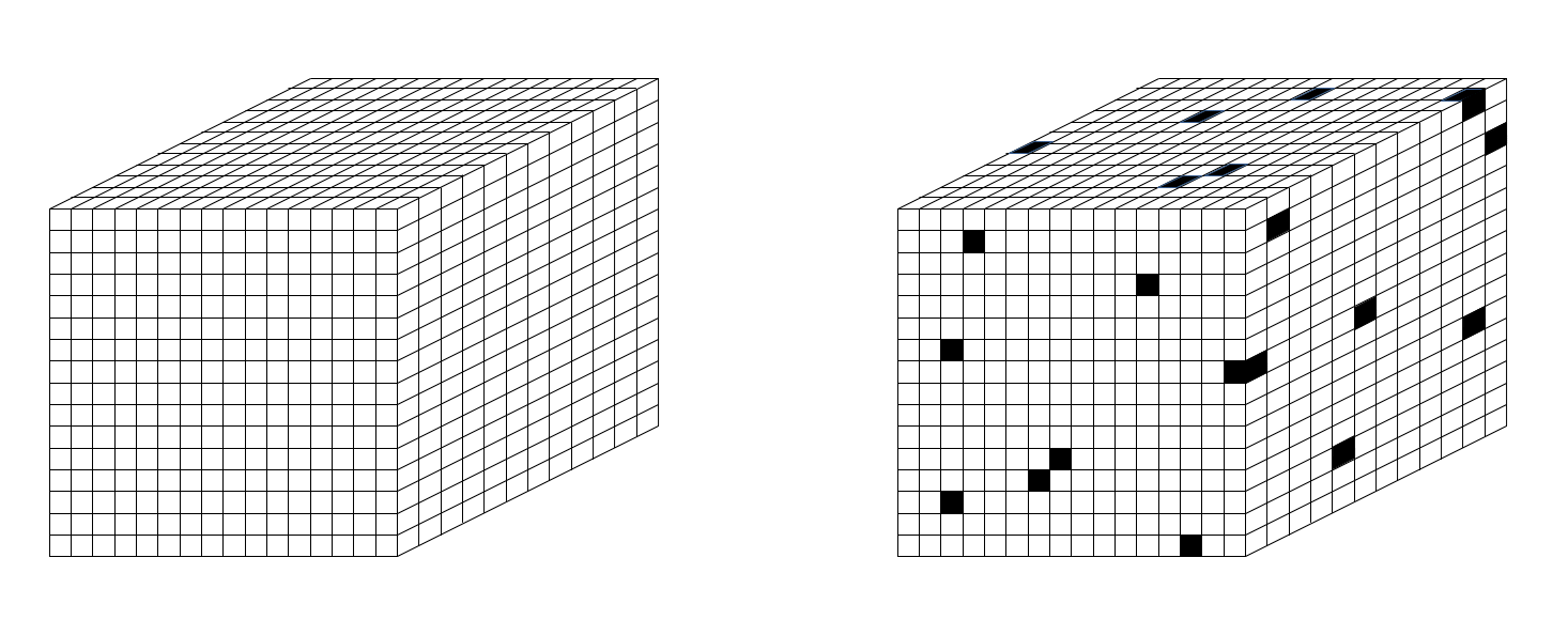
Now consider a cube of space, C, e.g., 8 Planck lengths on a side, as in Fig. 2. C is a bulk. C contains 512 planckons. Since they are binary, there are 2512 possible states of C. So, C can contain 512 bits of information. Now consider a layer of planckons that just wraps C. It consists of 6 x 64 = 384 planckons. That 1-Planck-cube-thick layer is the boundary, B, between C and the rest of the universe, U. It constitutes a communication channel between C and U. But B consists of only 384 planckons, so it has only 2384 states and so B can contain at most 384 bits.
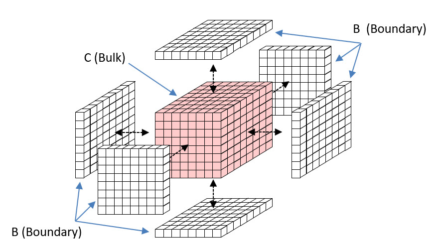
Suppose that a particular state (pattern), X, over the 512 bits (out of the 2512 possible patterns) exists. Now think of reading out the contents of C. That must occur as some instantaneous pattern over B’s 384 bits. So, no matter what actual pattern over C’s 512 bits actually exists, we can only read (at most) 384 bits from C. And similarly, we can only store at most 384 bits into C.
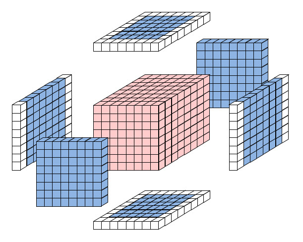
You might attempt to challenge my assertion that any read-out (or read-in) must be instantaneous. Why can’t we consider messages that take two (or more) time steps to send across the boundary (channel)? For example, suppose we imagine the cubes comprising B to be made of glass, so that you would just see the bit of C (the bulk) that is directly “under” the adjacent bit of B (the boundary), as in Fig. 3. There are 296 bits comprising the bulk’s outer layer: these are the rose-colored cubes. These could be seen through, i.e., copied to, B. But, how would any of the more deeply submerged cubes of the bulk be “seen” at B? You might imagine some temporal process by which the submerged bits of the bulk could be brought up next to the boundary. But the physical instantiation of any such “surfacing” process would require physical substrate. But, all 512 cubes (the totality of the bulk), is already accounted for in the pattern, X, itself. There are no additional bits available to build any such surfacing process (algorithm). So, we’re left with the conclusion that the amount of information that can be “seen in”, or extracted from, this bulk is upper-bounded by the number of bits comprising the boundary, i.e., the holographic principle. One cannot simply assume a physical, sequential process, allowing some kind of “surfacing” to read out the 512 – 296 = 216 submerged bits. One would have to describe the physical embodiment of any such process, and again, we’ve already used up all the bits in calculating the amount of information contained in the bulk.
I suppose we could consider allocating some fraction of the bulk’s 512 bits to representing that surfacing procedure. That’s worth exploring. But Bekenstein, Hawking, ‘t Hooft, and others have already shown that the amount of the information storable in a black hole (the densest possible bulk) is a 1/4 the area of its surface in Planck units, which is already several times lower than my simple argument would allow. This suggests finding such a partitioning, and accompanying description of the embodiment/operation of the surfacing algorithm, would be unlikely.
Conclusion
The pure concept of the holographic principle is that the maximum amount of information that can be stored in a volume is less than or equal to the amount of information that can be stored on its surface. This is highly counterintuitive. Indeed it is simply inconsistent with our everyday, macroscopic experience. But by making a few simple assumptions about the nature of the physical world, most importantly, that at the smallest scale, space itself is discrete, that units of space of this smallest size are binary, and that signaling is local, I construct a simple, classical explanation of why the holographic principle must be true.
Indeed, it’s a very simple argument. It does not require require the formalisms of quantum field theory (QFT) or string theory. But I have it on good authority that simpler explanations are better than more complicated ones 🙂 Some physicists have proposed the possibility that in the end, everything, i.e., this entire apparent (emergent) universe and all that happens in it, is just information, cf. Wheeler’s “It from Bit”. If so, then arguments like mine, or more generally, models in which states are ultimately just bit patterns and dynamics is just computational operations performed on bits, should be expected.