In quantum theory (QT), physical states are formally represented as vectors (in Hilbert space). As we all know, a vector is equivalent to a point, which is 0-dimensional, and therefore has zero extension. This suggests that any physical state, and thus any physical particle that is part of the ensemble present in that state, formally has zero extension. However, quantum theory avoids this interpretation by making the Hilbert space dimensions themselves, i.e., its basis vectors, be functions of space, not simply scalar-valued. Specifically, the value of any particular dimension is the absolute value of a wave function, i.e., of a particular probability density function over space. This is the mechanism by which quantum theory imparts spatial extent to physical entities. And it is central in facilitating the assertions by some quantum theorists that a purely formal mathematical object, i.e., a probability density function, used to represent a physical object is more real than the physical object itself. It’s also the underlying reason why in QT, all states that can exist actually do simultaneously exist, and furthermore, simultaneously exist at all instants of time. Somehow, they all occupy the same physical space, i.e., they all exist in physical superposition, and they do so for all of time. Make no mistake: quantum theory says that at every moment of time, all possible physical states exist in their entireties: in particular, QT does NOT say that any particular state partially exists. Rather, it says that the probability of actually observing any state, all of which fully physically exist, is what varies.

The choice to represent states as vectors can perhaps be considered the most fundamental assumption of QT. It implies that the space in which things arise and events occur exists prior to any of those things or events. This seems a perfectly reasonable, even unassailable assumption: indeed, how could it be otherwise? How can anything exist or anything happen unless there is first a space (and a time) to contain them? But that assumption is assailable. In fact, there is a simple formalism that completely averts the need for a prior space to exist. That formalism is sets. We can build dimensions, and therefore a space, out of sets. Specifically, a formal representation of dimension can be built out of, or emerge from, a pattern of intersections amongst sets, specifically amongst subsets chosen from a universe of elements, as explained in Fig. 1.

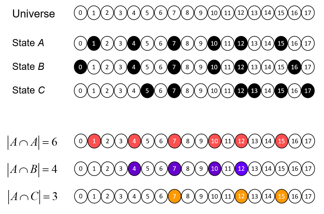
At top of Fig. 1, we show a universe of 18 binary elements. These elements happen to be arranged in a line, i.e., in one dimension. However, we’ll be treating the elements as a set: thus, their relative positions (topology) doesn’t matter; only the fact that they are individuals matters. Fig 1 then shows three subsets that represent, or are the codes of, three states, A-C, of this tiny universe, e.g., state A is represented by the set (code), {1,4,7,10,12,15}, etc. Thus, we will also refer to this universe as a coding field (CF). We assume that the codes of all states of this universe are subsets of the same fixed size, Q=6. The bottom portion of Fig. 1 shows the pattern of intersection of the three states with respect to state A. This pattern of intersection sizes imposes a scalar ordering on the states, i.e., a dimension on which the states vary. If we wanted, we could name this dimension, “similarity to A”. The pattern of intersections carries the meaning, “B is more similar to A than C is”. Thus, set intersection size serves as a similarity metric. No external coordinate system, i.e., no space, is needed to represent the ordering (more generally, similarity relation) over the states. The dimension is emergent. My 2019 essay, “Learned Multidimensional Indexes“, generalizes this to multiple dimensions.

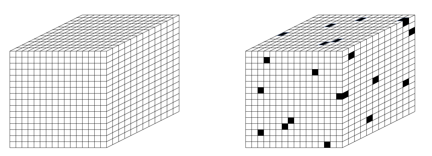
To be clear, my proposed set-based theory of physical reality does require the prior existence of something, but that something is not a (vector) space, but rather a set, i.e., a universal set. Specifically, I propose that the set of all physical units comprising the universe is the set of Planck-length (10^-35 m) volumes that tile the physical universe, as in Fig. 2 (left). So let’s call these quanta of space, planckons. N.b.: Figs. 2 thru 4 depict the set of planckons as tiling a 3-space, i.e., as “voxels”. However, the 3D topology is not used in the proposed model’s dynamics: the rule for how the state evolves does not use the relative spatial information of the planckons. As described herein, the apparent three spatial dimensions of the the universe, and any other observables, emerge as patterns of intersection over sets chosen from that underlying set of planckons, and as temporal patterns of evolution of those patterns (e.g., to explain movement through apparent macroscopic spatial dimensions). So to emphasize, Planckons do not move. Furthermore, the set of all planckons is partitioned into two sets, one being the underlying physical reification of matter, the fermionic planckons, or “flanckons“, and one being the underlying physical reification of forces (i.e., of transmission of effects, i.e., of signals), the bosonic planckons, or “blanckons“. The two partitions are intercalated at a fine scale, many orders of magnitude below that probed by experiment thus far (described shortly). And furthermore, planckons are binary-valued: at any time T, a planckon is either “active” (“1”) or “inactive” (“0”). For the case of blanckons, “active/inactive” can be viewed as representing the weight of a connection, 1 or 0, as in a binary weight matrix. I propose that in any local region of space (defined below), the matter and force content at T is present as a sparse subset of the flanckons being active, as suggested in Fig. 2 (right), though this picture is refined in Figs. 3 and 4. In fact, the proposed sparseness is many orders of magnitude greater than Fig. 2 (right) suggests.

Before continuing with the set-based physical theory, let me say that it was first, and still is foremost, a theory of how information is represented and processed in the brain (specifically in cortex). I am a computational neuroscientist, not a physicist, and the key insight underlying that theory, called Sparsey, is that all items of information (informational entities) represented in the brain are represented as sets, specifically sparse sets, of neurons (formalized as having binary activation), chosen from the much larger population (field) of neurons comprising a local region of cortex.¹ Sparsey and the analogy between it and the set-based physical theory was described in some detail in my earlier essay, “The Classical Realization of Quantum Parallelism”. The explanations of superposition and of entanglement given in that earlier essay and which will be improved in part 2 of this essay come as direct, close analogs from the information-processing theory. In fact, the only difference between the two theories is that in the information-processing version, the elements comprising the underlying set from which the codes of entities (i.e., percepts, concepts, memories), and of spatial/temporal relationships between entities (i.e., part-whole, causal, etc.) are drawn are taken to be bits (as in a classical computer memory), whereas, in the physical theory, the elements comprising the underlying set are “its“, or as we’ve already called them, planckons, cf. Wheeler’s “It from Bit” (discussed here).

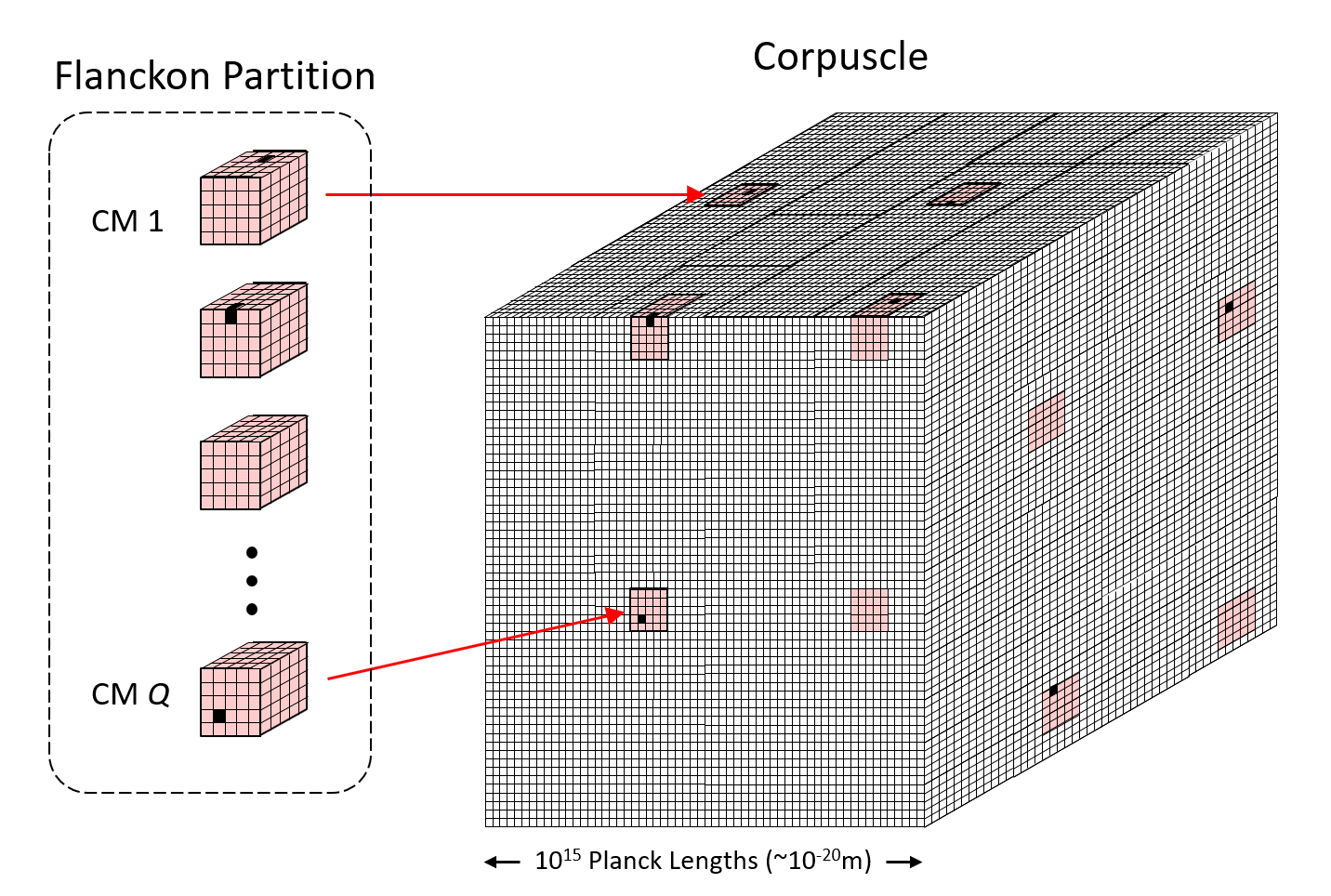
In focusing now on the physical theory, the first order of business is to refine Fig. 2, in particular, to define a local region of space, which is the fundamental functional unit of space, called a “corpuscle“, and describe how it consists of a fermionic and a bosonic partitions. By fundamental functional unit of space, I specifically mean the largest completely connected volume of space, which will be explained in the next few paragraphs. Fig. 3 (right) shows a “corpuscle“, which, for concreteness, we can assume to be a cube, 10¹⁵ Planck lengths, or roughly, 10^-20m, on a side, thus far smaller than the smallest distance directly measured experimentally thus far (10^-18m). It consists of two partitions:

1. Flanckon partition: representing the fermionic, i.e., matter, state of the corpuscle; and
2. Blanckon partition: representing the transitions from one matter state of the corpuscle to the next or to the next state of a neighboring corpuscle. Thus, this partition represents the bosonic aspect of reality, i.e., transmission of effect, or operation of forces.

The flanckon partition is far smaller, i.e., consists of far fewer planckons, than the blanckon partition and it is embedded (intercalated) sparsely and homogeneously throughout the corpuscle, i.e., throughout the far larger blanckon partition. Fig. 3 (left) shows the corpuscle’s flanckon partition “pulled out” from corpuscle, revealing its sub-structure, namely that it consists of Q winner-take-all (WTA) competitive modules (“CMs“) (shaded rose), each comprised of K flanckons. N.B.: While the CMs are depicted as being only 5 Planck lengths on each side in this figure, we assume they are far larger, e.g., 10⁵ Planck lengths on each side, thus containing 10¹⁵ flanckons. These CMs are dispersed sparsely and homogeneously throughout the corpuscle’s far larger number of blanckons (white) as shown in Fig. 3 (right).² The matter state of the corpuscle is defined as a set of Q active flanckons (black), one in each of the corpuscle’s Q CMs. N.B.: The fact that the CMs act as WTA modules, where exactly one of its flanckons can be active (“1”) at any time, T, is an axiom of the theory. Also note that in the figures, CMs without a black flanckon can be assumed to have one active flanckon at some internal position.

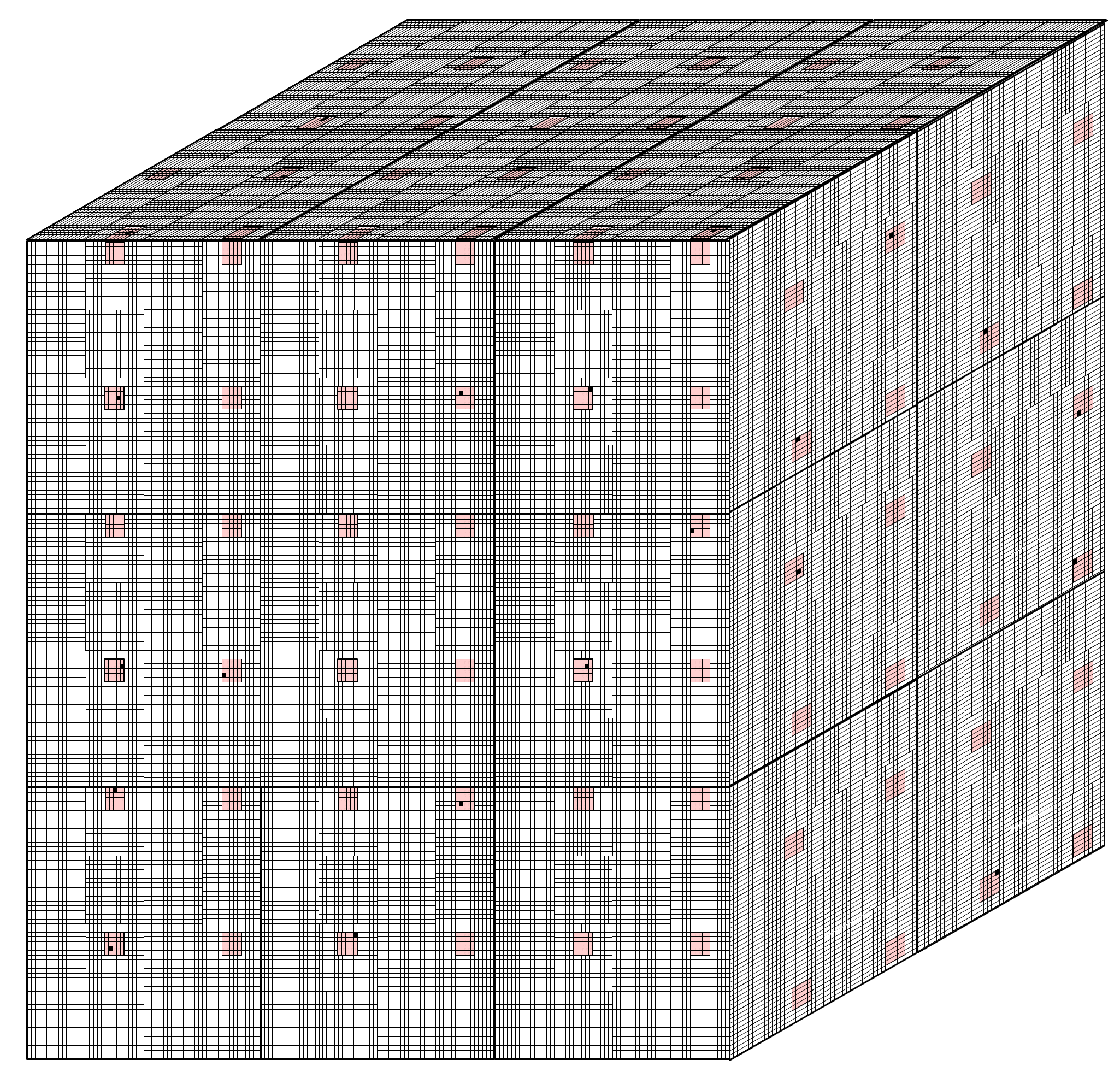
As stated above, the blanckon partition provides the means by which effects (signals, forces) can be transmitted from a corpuscle’s matter state at T, both recurrently to its own state at T+1, as well as to the six neighboring, face-connected corpuscles (the universe is hypothesized to be a cubic tiling of corpuscles as shown in Fig. 4) at T+1. Given that the matter state of every corpuscle is a sparse activation pattern over a set of N = Q x K flanckons (again, which are binary valued), in order to instantiate any possible transition, i.e., mapping, from the matter state of a corpuscle at T, either recurrently to itself or to a neighboring corpuscle, at T+1, we require the corpuscle’s flanckon partition to be completely connected to itself and to its neighbors. Thus, if the corpuscle contains N flanckons, then it must contain at least 7 x N² blanckons, a matrix of N² blanckons for the recurrent matrix to itself, and a matrix of N² blanckons connecting to the flanckons in each its six face-connected neighboring corpuscles. So this is what I meant above by the corpuscle being “the largest completely connected volume of space”: it is the largest volume of space for which dynamics, i.e., transitions from one state to the next, in both that volume and its neighbors can be a total function (of the prior state).³ In particular, no volume consisting of two of more corpuscles can be completely connected. Being the largest volume of space for which the time evolution of state is a total function, the corpuscle is the natural scale for defining the states and dynamics of universe, justifying referring to the corpuscle as the fundamental functional unit of space.

The space of possible matter states of this fundamental region of space is the number of unique sets of active flanckons in the corpuscle, which is K^Q (again, flanckon partition is organized as Q CMs, each with K flanckons, exactly one of which is active at any T). For example, if Q = 10⁶ and K = 10¹⁵ (because we assumed above that the CMs are actually 10⁵ Planck lengths on each side), then the number of unique matter states specifiable for the corpuscle, which again, is a cube of space only 10^-20m on a side, is 10^15,000,000. The transitions between states of a single corpuscle are specified in the binary pattern over that corpuscle’s recurrent blanckon matrix. This pattern of binary weights of the corpuscle’s recurrent blanckon matrix instantiates the operation of physical law, i.e., the dynamics (of all forces), for the individual corpuscle, which, again, is the fundamental functional unit of space. The weight pattern of this recurrent blanckon matrix in conjunction with those of the other six blanckon matrices (one to each of the six neighboring corpuscles), fully specifies the operation of physical law at all scales throughout the universe. That is, all effects are local: there is no action at a distance. Note: While the pattern over a corpuscle’s flanckon partition, i.e., its matter state, will generally change from one moment to the next, the pattern over the blanckons, again, which instantiates physical law, is fixed through time.

What do we mean by “instantiate physical law”. In the first place, we mean that the state transitions determined by the blanckon matrix are consistent with macroscopic observations, e.g., that a state at time T, in which a body is moving with speed s in some direction, will transition to a state at T+1, in which that body is at a new location along the line of motion and determined by s. The larger is s, the further the body is in the state at T+1. In other words, the transitions must exhibit the the kind of smoothness, or spatiotemporal continuity, that characterizes macroscopic physical law, not just for inertial movement, but for the macroscopic manifestations of all physical forces.⁴ Yet another way of stating this criterion is that the transitions must bring similar initial states into similar successor states, or in yet other terms, that the blanckon partition (which is a effectively a set of seven completely connected binary weight matrices, a recurrent one and six bipartite ones connecting to the six adjacent corpuscles) must preserve similarity. As explained with respect to Fig. 1, since states are represented as (extremely sparse) sets, the natural measure of similarity is intersection size.

Given that each of the possible matter states of a corpuscle is represented by a set and that more similar states will be represented by more highly intersecting sets, the essential question for the theory becomes:

• Is the set of corpuscle states needed to explain all observed (i.e., possible) physical phenomena small enough so that the corpuscle’s blanckon matrix can produce all state transitions subsumed in the set of all possible physical phenomena?

That is, two similar states, S1 and S2, will have many of their flanckons in common. Since the blanckon partition (binary weight matrix) is permanently fixed, whenever either state occurs, that common set will send the same signals via the blanckon partition. While the non-intersecting portion of either state will send different signals via the blanckon partition in any such instance, we must specify a disambiguating mechanism by which the correct successor state reliably, in fact deterministically, occurs in both instances, i.e., despite the “crosstalk” interference imposed by the set of flanckons common to S1 and S2. Such a disambiguating mechanism was first explained in the context of the information-processing version of this theory, Sparsey, in my 1996 thesis, and many times since, and need not be described here again in detail. The reader can refer to those earlier works for the detailed explanation. The thesis in particular, showed that a large number of state transitions can be embedded in a single, fixed binary matrix. We now develop insight suggesting that for a volume of space as small as we hypothesize for the corpuscle, i.e., 10^-20m on a side, the number of possible physical states needed to explain all higher-level phenomena might not be that large. The vast richness of variation observed at macroscopic scales might plausibly be produced by a relatively small canonical set of states, and a correspondingly small set of transitions, at the fundamental functional scale, i.e., the corpuscle scale, of the universe. Of course, stated this generally, such distillation is the goal of all science, especially physics, both classical and quantum. However, it is the dynamics in particular, i.e., the rules for how state changes, that is explicitly reduced to a small number in the edifice of science thus far. The range of states to which the the small number of rules can be applied has always been conceptualized as essentially infinite. In stark contrast, the claim here is that the underlying number of fundamental (matter) states is in fact discrete and relatively small. And the number of rules, i.e., of fundamental transitions is also discrete and relatively small, though substantially larger than in mainstream approach of science thus far.

So, on to discussing the plausibility of the assertion that only a relatively small number of fundamental matter states are needed for the corpuscle. At the outset, we acknowledge that the range of physical phenomena at the macroscopic scale appears vastly rich, and has historically been considered to vary continuously on any macroscopic dimension. However, we have no direct experience of the possible range of variation or of the granularity of variation at the scale of the corpuscle, 10^-20m. Thus, from a scientific point of view, the number of fundamental matter states needed at the corpuscle scale (in order to account for all higher-level physical phenomena) is an open question. After all, the corpuscle is smaller than any distance ever measured (observed) thus far. In fact, while the fundamental particles of the Standard Model (SM), are generally treated as point masses, and thus being of zero size (again, the equivalence of vectors and points), the composite particles, in terms of which numerous experimental phenomena are described are assigned sizes far larger than the corpuscle. For example, a proton is estimated to be 10^-15m in diameter, five orders of magnitude larger than the corpuscle, and the “classical radius of the electron” is also 10^-15m (see here). Thus an individual proton (or electron) spans a diameter of 10⁵ corpuscles. While it is possible that SM-scale particles can physically overlap, we will assume that at the scale of the corpuscle, they cannot.⁵ Thus, we assume that the number of unique particles that can be present in the corpuscle is the number of fundamental particles in the SM, which allowing for anti-particles, we’ll approximate as 100. We then have the question of how these particles might be moving through a corpuscle. How might we quantify momenta? If some of these particles have size larger than a corpuscle, we’re talking about quantifying the movement of the centroid of a particle through a corpuscle (not of an entire particle within a larger space).

So, the specific question we have is: for any of these 100 particles, how many discrete velocities (of its centroid) through the corpuscle are needed in order to explain the apparently continuously varying velocities of these particles at macroscopic scales? And since the mass is fixed by particle type, the set of velocities will determine a corresponding set of momenta. So our question is how many velocities are needed, i.e., how many combinations of direction and speed. One might immediately think that the number of unique velocities is infinite. However. we have already assumed that space is a cubic tiling of the fundamental functional units of space (corpuscles). In this case, there are only 6 canonical directions that a particle’s centroid can take through the corpuscle. Thus, we’ve reduced what, in the naive continuous view of macroscopic space, is an infinity of possible directions to just six canonical directions, left, right, up, down, forward, backward, at the corpuscle scale.

So, what about speed? How many unique speeds are needed, again, to explain all observed speeds of higher-level particles/bodies? To answer, first of all note that since space is discrete (a cubic tiling of Planck volumes), velocity immediately becomes discrete-valued, i.e., a particle’s centroid can only move by some discrete number of Planck lengths in any given time unit. As stated earlier, we assume the size of the corpuscle is 10¹⁵ Planck lengths on a side. Recall, the Planck length is defined as the distance light travels in one Planck time (~10^-43s). Suppose we then define the fundamental time delta, T, of the universe, i.e., the rate at which corpuscle state is updated, to be equal to the time light would take to traverse the corpuscle, i.e., 10¹⁵ Planck times (10^-28s, thus orders of magnitude shorter than the shortest duration experimentally observed thus far). Thus, an initial hypothesis could be that 10¹⁵ unique speeds are possible. For example, considering a strictly rightward movement, upon entering the left side of a corpuscle at T, a particle’s centroid could move by one Planck length by T+1, or by two Planck lengths, etc., or by up to 10¹⁵ Planck lengths (the right side of the corpuscle) by T+1. No faster speed is possible, i.e., the particle cannot arrive in the next corpuscle to the right in the interval T, since that would imply moving faster than light.

But do we actually need all 10¹⁵ of those speeds in order to account for all observed speeds (of fundamental particles, or anything larger)? Probably not. Perhaps we need only a relatively tiny number of unique speeds through a corpuscle, perhaps even just a few, in order to account for the apparently continuous valuedness of speed and velocity at macroscopic scales. Fig. 5 explains why a small number of possible speeds at the corpuscle level can produce a vastly more finely graded set of possible speeds in distant corpuscles. In this figure, we depict space as being only 2D. Each column depicts one possible sequence of discrete rightward movements of a particle’s centroid across four corpuscles (red boxes, each is 10^-20m on a side). Each corpuscle is divided into 4×4=16 sectors. This indicates the assumption that there are only four possible non-zero speeds that a particle can have, 1/4 c, 1/2 c, 3/4 c, and c. Actually since we are talking about speeds of matter particles, the top speed is something near but less than c. Thus in column one, the particle (it’s centroid) enters at the left side of the leftmost corpuscle at T=1. It then has zero speed until T=7 (again, each T delta is 10^-28 s), whereupon it moving by two sectors per T delta, or 1/2 c. It’s final speed, measured over the total duration, and across the macroscopic (as in spanning multiple, i.e., 4, corpuscles) expanse is 1/6 c. Column two shows the case of the particle moving at the constant speed of 1/4 c across the macroscopic expanse. Columns three and four show other overall macroscopic speed measurements and column five shows a particle moving at c, or again, at just below c (please tolerate the slight abuse of graphical notation here). So, even assuming only four non-zreo speeds at the corpuscle scale, these five columns show just a tiny subset of the total number of unique speeds that could be represented over even the tiny distance of four corpuscles. The number of unique speeds that are possible, assuming only four non-zero speeds, over distances spanning even the size of a single proton, 10^-15m = 10⁵ corpuscles, is truly vast. No experiment result thus far will have been able to distinguish speed being a truly continuous variable from speed being discrete but of vast granularity.

Suppose then that we, more conservatively, assume there are 10 unique speeds at the corpuscle scale. And, as stated above, given our assumption that space is a cubic tiling of corpuscles, there are only six possible directions of movement through a corpuscle. Thus, there are only 60 possible velocities at the corpuscle scale. In this case, we have 100 fundamental particles times 60 fundamental velocities, or just 6,000 fundamental “matter states” for a corpuscle. Furthermore, we assume that at this corpuscle scale, these motions are deterministic. That is, each of the 6,000 states of a corpuscle, X, leads to a particular definite successor state in X, via the recurrent, complete blanckon matrix, and to definite successor states in each of X’s six face-connected neighboring corpuscles, via the six corresponding complete blanckon matrices to those corpuscles. In other words, each of these matrices only needs to embed 6,000 transitions. The question we then have for any of these seven blanckon matrices is:

• Given that each state is a set of 10⁶ active flanckons chosen from a corpuscle’s flanckon partition of 10²¹ flanckons (in particular, from a space of 10^15,000,000 unique active flanckon patterns), and the matrix consists of 10²¹ x 10²¹ = 10⁴² blanckons, can we find a set of 6,000 such flanckon patterns such that their intersection structure reflects the similarity structure over the physical states and each pattern can reliably (absolutely) give rise to the correct, i.e., consistent with macroscopic dynamics, successor states in the source corpuscle and in its six face-connected neighbors?

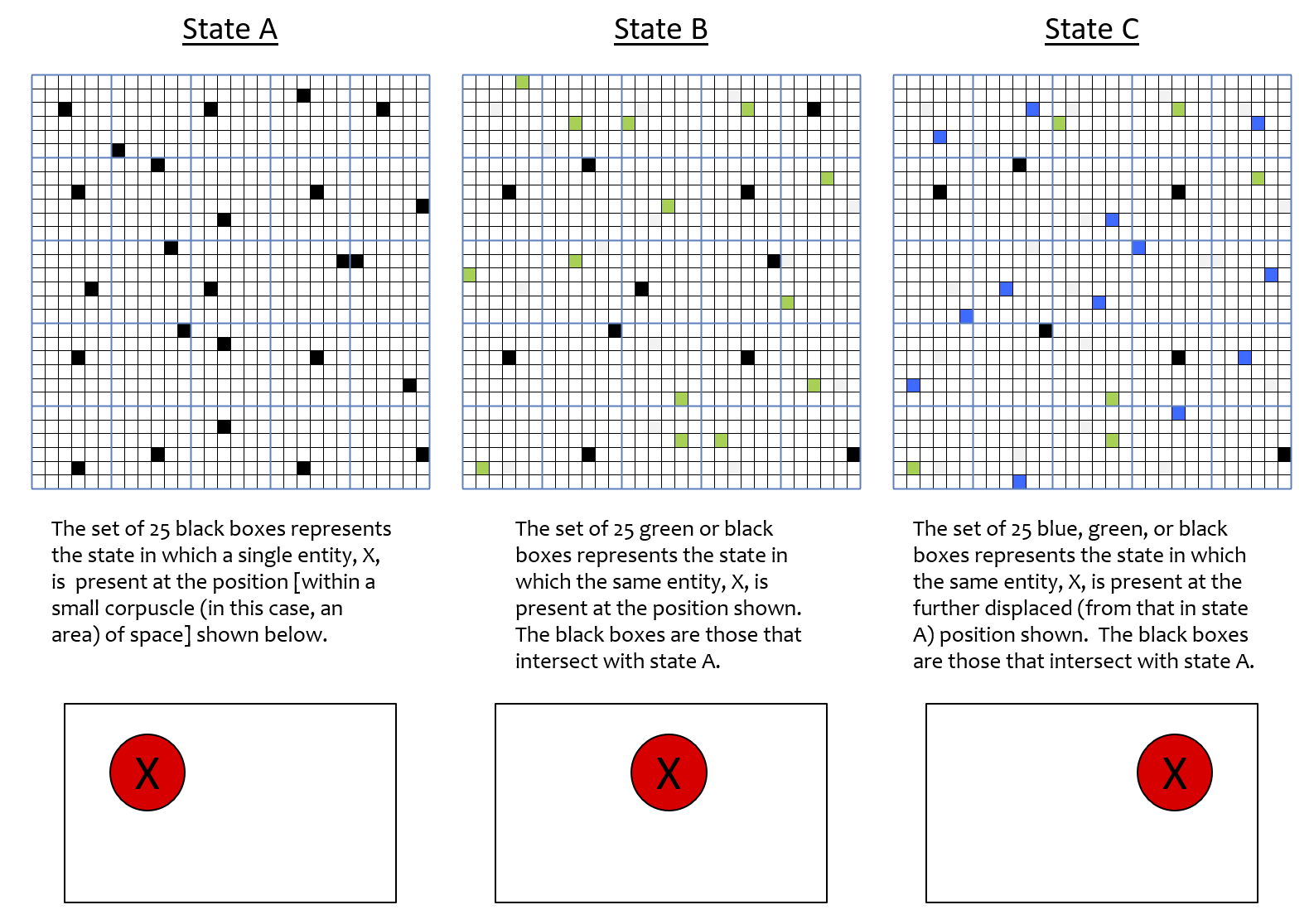
We believe the answer is quite plausibly yes, and the prior works describing Sparsey’s memory storage capacity provides preliminary evidence supporting this, since Sparsey’s representational (data) structure is identical to the physical representation described here. In fact, Fig.1 and its explanation already provided a basic construction and intuition for why the answers to these questions might be yes. The simple case of Fig. 1, where the set elements were organized in 1D, allowed us to give an exact quantitative example of how dimension, and thus similarity on a dimension, can emerge as a pattern of intersections. Visually depicting the same quantitative tightness in the 3D case is very difficult. However, Fig. 6 presents a quantitatively precise example for the 2D case. It should be clear that the same principle (i.e., patterns of intersection) extrapolates to 3D as well. In Fig. 6, the corpuscle is 2D and organized as 25 CMs (blue lines), each composed of 36 flanckons. N.b.: In Figs. 6 and 7, we explicitly depict only the flanckon partition of the corpuscle! The first column shows a state, A, of the corpuscle, which we will deem to represent the presence of an electron, X, having the depicted location within the corpuscle (red circle)⁶ The middle column shows state B, in which X is at a position relatively near that in state A. The last column shows another state, C, in which the X has a position further away from its position in A. In each case, the state is represented by a set of Q=25 co-active flanckons, i.e., a code. These codes have been manually chosen so that the pattern of intersections correlate with the three positions. That is, B’s code (the union of black and green flanckons) has 11 flanckons (black) in common with A’s code and C’s code (the union of black, blue and green flanckons) has 6 flanckons (black) in common with A’s code. This pattern of intersections correlates in a common sense fashion with the distance relations amongst the three positions, i.e., intersection size decreases directly with spatial distance. Whereas in the analogous 1D example of Fig. 1, we suggested that we could call the dimension represented by the pattern of intersections, “similarity to A”, the greater principle is that a pattern of intersections can potentially represent any observable, which here, we suggest is “position”, or perhaps more specifically, “left-right position” in the corpuscle.

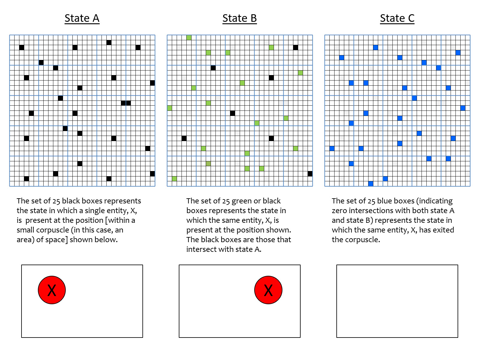
In fact, if the three states of Fig. 6 were to occur sequentially in time, then we could also assert that this same pattern of intersections also corresponds to a particular velocity across space, and since X is an electron, a particular momentum. One can imagine different sets (activation patterns) for states B and C, that would correspond to the same particle but moving at a faster velocity. Fig. 7 shows one such possible choice of states B and C. Specifically, the intersection of states A and B is smaller (than in Fig. 6) and state E has zero intersection with A or with B. The zero intersection naturally corresponding to the reality that at this faster speed, the particle is no longer present in the corpuscle. State E of Fig. 7 corresponds to a state with no particle present, i.e., the “ground state”. It is an open question whether the ground state of a corpuscle needs to be explicitly represented by a particular activation pattern of the flanckons or could be represented by the zero activation pattern, i.e., no active flanckons.

Figs. 6 and 7 raise a key question: how many gradations along any such emergent dimension can be represented in a corpuscle? Or more generally, how many dimensions (observables) can be represented, and with what number of gradations on each of them? In this example, all codes are of size Q=25. Therefore the range of possible intersection sizes between any two codes is 26. Thus, if the only variable (observable) that needed to be represented for the corpuscle was left-right position of (what would then have to be only) a single entity, we could represent 26 positions. Furthermore, in this case, no other information, i.e., about any other variable, e.g., entity size, or entity identity, charge, spin, etc., could be represented. Note however that for the case of 3D corpuscles, where we assumed a corpuscle contains 10⁶ CMs, there are 10⁶+1 levels of intersection, which could represent that many gradations on a single dimension, or could be apportioned out to some number of dimensions.

But Fig. 6 raises an even more important point: We’ve suggested that a pattern of intersections can represent spatial position varying across the left-right extent of the corpuscle. Yet clearly, all possible codes that could be chosen (there are 36²⁵ of them) will be approximately homogeneously diffusely spread out across the full extent of the corpuscle (enforced by the theory’s rule that all codes must consist of exactly one active flanckon per CM), and thus have approximately the same centroid, i.e., the centroid of the corpuscle. Thus, we can begin to see how a macroscopic observable such as position might be considered an illusion, or a construction, at least over the scale of a single corpuscle. The question then arises: if one accepts the possibility that merely different sets, all of which have almost the same centroid (in any physical reification of the set elements), can manifest as different positions (across the extent of the corpuscle), to what is this manifesting done? That is, where is the observer? The answer is that the observer is, in principle, any corpuscle on the terminal end of a connection matrix leading from the subject corpuscle. In fact, the “observer” could even be the subject corpuscle, i.e., receiving signals at T+1 originating from its own state at time T, via the recurrent matrix (of blanckons). There is no need for the “observer” to be any sort of conscious entity: any part of the universe, i.e., any corpuscle, that receives signals (a.k.a. energy, influence) from any other corpuscle (or from itself) is an “observer”.

In part 2 of this essay, I’ll focus on the blanckons and propagation of signals between corpuscles and across time steps. But even in that scenario, it remains the case that none of the underlying fundamental constituents of reality, i.e., the planckons, move. Just as the appearance of (an entity being located at) different positions across the extent of a corpuscle can be explained in terms of the pattern of intersections over codes, the appearance of smooth movement of an entity through a sequence of positions across the extent of a corpuscle can be explained as the sequential activation of said codes in the order in which said intersections are seen to be active. And, all that is needed in order for that smooth movement to appear to continue across an adjacent corpuscle is that there exist codes in that corpuscle whose pattern of intersections can also be interpreted as representing that continued motion. Nothing actually moves in the set-based theory; there is just change of activation patterns from one moment to the next, just is as the case for the pixels of the TV when you watch television.