Quantum theory (QT) is based on vectors. In QT, the physical system (world) is represented as an infinite-dimensional Hilbert space. The space is ontologically prior to the stuff, i.e., matter and energy, or fields if you like, that exists in the space. Each state of the system is defined as a point in the Hilbert space. Thus, the space of QT, i.e., the Hilbert space itself, is definitely not emergent. In the theory I describe here, there is also something that exists prior to the stuff. But it is not a vector (tensor) space. It’s just a set, a collection of unordered elements. These elements are the simplest possible, just binary elements (bits) that can be active (“1”) or inactive (“0”). Instead of the states being defined as points in a space, they are defined as subsets, very sparse subsets, of the overall, or universal, set. More precisely, I will define the matter (fermionic) states of the physical system as these sparse subsets. Thus, I will call this universal set the fermionic field. My theory will be able to explain the existence of individual matter entities (fermions) moving and interacting in lawful ways but these entities and the space within which they apparently move/interact will be emergent, i.e., epiphenomenal. In fact, any one dimension of the emergent space will be explained as the combination of: a) a pattern of intersections that exists over the sets that define the fermionic states of the system; and b) the sequential patterns of activation of those intersections through time.
In addition to the fermionic field, my theory also has a complete recurrent matrix of binary-valued connections, or weights, from the set of bits comprising the fermionic field back to itself. It is this matrix that mediates all changes of state from one time step to the next, i.e., the system’s dynamics. In other words, it is the medium by which effects, or signals, propagate. Thus, I call it the bosonic field. Note that my theory’s mechanics, i.e., the operation (algorithm) that executes the dynamics, is simpler, more fundamental, than any particular force of the standard model (SM). My theory has the capacity to explain, i.e., mechanistically represent, any force, i.e. any lawful pattern of changes of state through time. In fact, any such force will also be emergent: as suggested above, the fermionic evidence of any instance of the application of any force will be physically reified as a temporal sequence of activations of intersections. And the actual physical reification of the force at any given moment is the set of signals traversing the matrix from the set of active fermionic bits at t (which arrive back at the matrix at t+1). Thus, in this theory, nothing actually moves. That is, neither the fermionic nor the bosonic bits move. They change state, i.e., activate or deactivate, but they don’t move. All apparent motion of higher-level, e.g., standard model (SM) level, fermions and bosons, is explained as these patterns of activation/deactivation. We’re all very familiar with this concept. When you watch TV and see all the things moving/interacting, none of the pixels are actually moving. They’re just changing state.
As will become apparent, in my theory, the underlying problem is: can we find a set of state-representing sets and a setting of the matrix’s weights that implement (simulate) any particular emergent world, i.e., any given emergent space, in general, having multiple dimensions, some of which are spatial and some not, and multiple fermionic entities? This can be viewed as a search problem through the combinatorially large space of possible sets of state-representing sets and weight sets. The way I’ll proceed in describing this theory is by construction. I’ll choose a particular set of state-representing sets. I’ll choose them so that they have a particular pattern of monotonically decreasing intersections. Thus, that pattern of intersections constitutes a representation of a similarity (inverse distance) relation over the states. I’ll then show that there is a setting of the weights of the matrix, which, together with an algorithm (operator) for changing/updating the state, constrains the states to activate in a certain order, namely an order that directly correlates with the intersection sizes. Thus, the operator enforces gradual change through time of the value of that similarity (inverse distance) measure, i.e., it enforces locality (local realism) in the emergent space.
The Set-Based Theory
It is possible to represent the states of a physical system as sets, in particular, as sparse sets over binary units, where all states are of the same cardinality Q. Fig. 1 shows four states, A-D, represented by four such sets, ψ(A)-ψ(D). Here the representational field (the universal set), F, is organized as Q=16 winner-take-all (WTA) modules each with K=36 units. All state-representing sets consist of Q active units, one in each of the Q modules.
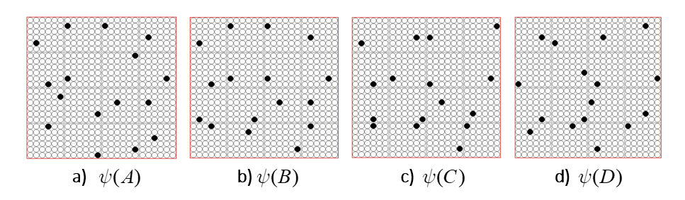
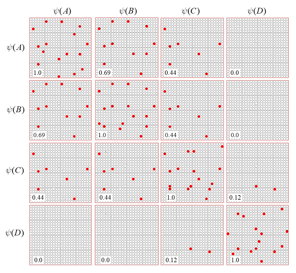
It is possible to represent the similarity of states by the size of their intersection. I’ve chosen these four sets to have a particular pattern of intersections, as shown in Fig. 2: specifically, the sets representing states B, C, and D, have progressively smaller intersections (red units) with the set representing A. Thus, this similarity measure, which we could call “similarity to A”, is physically reified as this pattern of intersections.
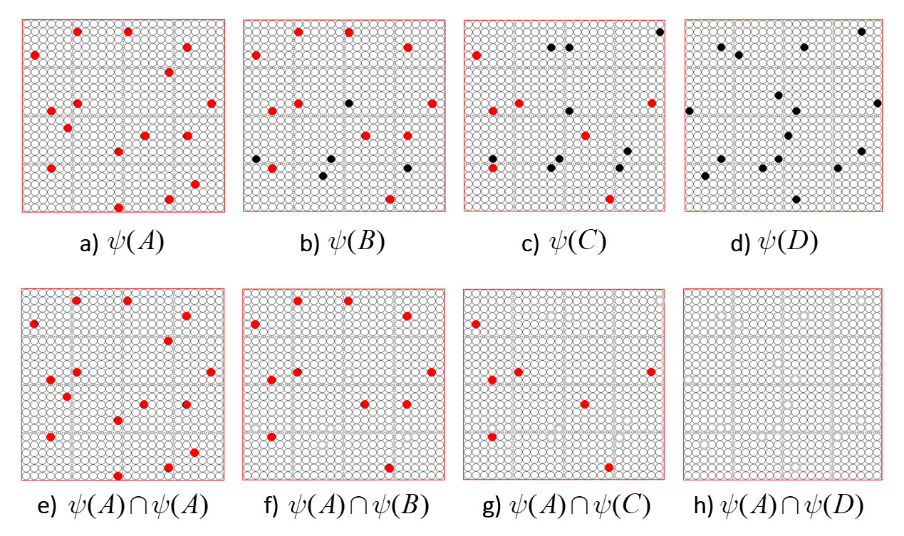
ψ(A) highlighted in red. (bottom row) Just showing the intersecting units.
We can imagine a method for reading out the value of this similarity measure. Specifically, we could have another field of binary units, a simpler field, with just four units, labelled, “0”-“3”, that receives a complete binary matrix from F. Suppose we activate state A, i.e., turn on its Q units, i.e., the set ψ(A), and at the same time, turn on the output unit “0”, and increase the Q weights from the Q active units to output unit “0”, as in Fig. 3a. Suppose that at some other time, we activate B, i.e., ψ(B), simultaneously turn on output unit “1”. and increase the Q weights from ψ(B) to “1”, as in Fig. 3b. We do this for states C and D as well, increasing the Q weights from ψ(C) to “2”, and the Q weights from ψ(D) to “3”, as in Figs. 3c,d.
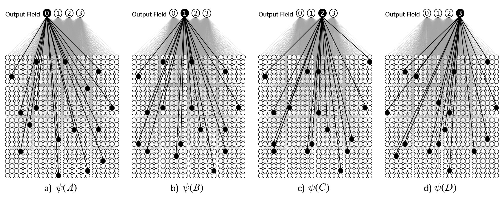
Now, having done those four operations in the past, suppose state A again comes into existence, i.e., the set ψ(A) activates, as in Fig. 4a. In this case, because of the weights we increased in that original event in the past (in Fig. 3a), the input summation to output unit “0” will be Q=16, output unit “1” will have summation |ψ(A)∩ψ(B)|=11, “2” will have sum |ψ(A)∩ψ(C)|=7, and “3” will have sum |ψ(A)∩ψ(D)|=0. Suppose we treat the output field as WTA: then, “0” becomes active and the other three remain inactive. In this case, the output field has indicated, i.e., observed, that the physical system is in state A. Note that these summations are due to (caused by): a) the subsets of units that are the intersections of the relevant states; and b) the pattern of weight increases that have been made to the matrix. And note that that pattern of weight increases is necessarily specific to the choices of units that comprise the four sets, ψ(A)-ψ(D).
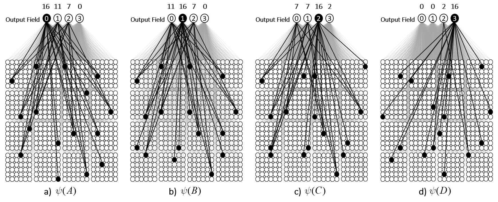
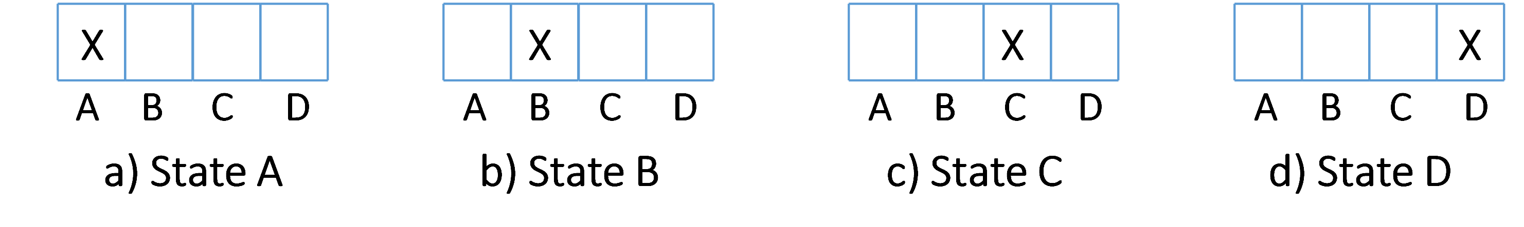
Thus far, I’ve said only that these four states have a similarity relation that correlates with their representations’ intersection sizes. But let’s now get more specific and say that these four sets represent the four possible states of a very simple physical system, namely, a universe with one spatial dimension with four discrete positions, A-D, and one particle, x, which can move from one location to an adjacent one on any one time step, as in Fig. 5. Thus it has two properties, location and some basic notion of velocity. In this case, state A can be described as “x is at position A” or “x is distance 0 from A”, state B can be described as “x is at position B”, or “x is distance 1 from A”. Thus, the output unit labels in Figs. 3 and 4 reflect the distances from A. If x was in position A at t (i.e., Fig. 5a) and position B at t+1, then we could describe Fig. 5b as “x is in at position B, moving with speed 1”.
Now, suppose that instead of the output field functioning as WTA, we allow all its units to become active with strength proportional to their input sums normalized by Q. Then unit “0” is active at strength 16/16=1, unit “1” is active at strength 11/16 ≈ 0.69, unit “2” is active with strength 7/16 ≈ 0.44, and unit “3” at strength 0/16 = 0. The vector of output activities constitutes a similarity distribution over the states. And, if we grant that similarity correlates with likelihood, then it also constitutes a likelihood distribution. Furthermore, we could easily renormalize this likelihood distribution to a total probability distribution (by adding up the likelihoods and dividing the individual likelihoods by their sum). We can do the same analysis for each of other three states and the summations will be as shown at the top of Figs. 4b-d. Fig. 6 shows the complete pairwise intersection pattern of the four states (sets). The numbers show the fractional activation (likelihood) of a state when the state along the main diagonal is fully active. In all cases, we could normalize these distributions to total probability distributions, which would comport with the physical intuition that given some particular signal (evidence) indicating the position of a particle, progressively further locations should have progressively lower probabilities.
The State Update Operator
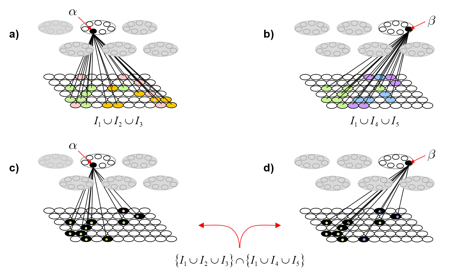
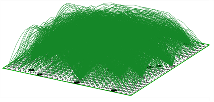
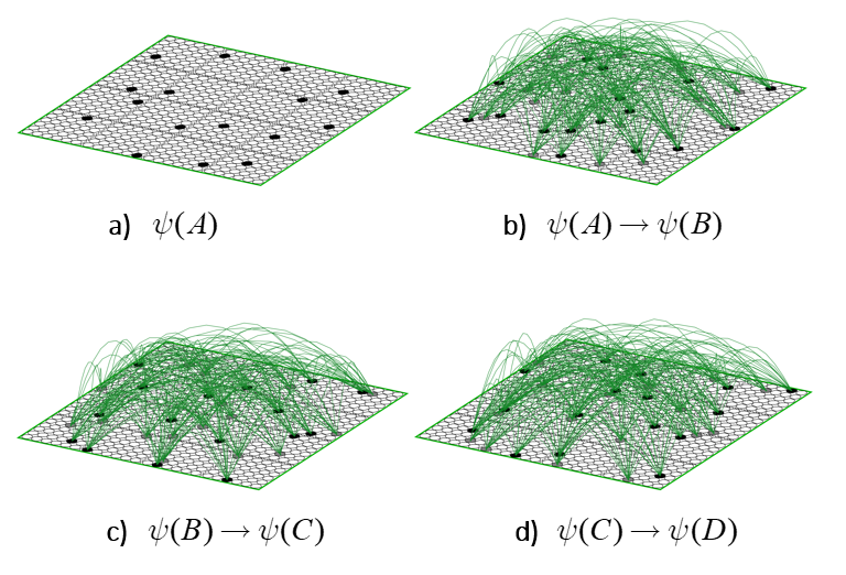
The simple example of Figs. 1-6 provides a mechanistic explanation of how a pattern of set intersections can represent, in fact, physically reify, a similarity measure, i.e., inverse distance measure, or in still other words, a dimension. But something more is needed. Specifically, in order for this dimension to truly have the semantics of a spatial dimension, there must be constraints on how the state can change through time. In Figs. 3 and 4, I’ve introduced a weight matrix to read out the state. But thus far I’ve provided no mechanism by which the state itself can change through time. Thus, we need some kind of operator that updates the state. And, this operator must enforce the natural constraint for a spatial dimension which is that movement along the dimension must be local. This is fundamental to our notion of what it means to be a spatial dimension. If, from one time step to the next, the particle could appear anywhere in the universe, then there is no longer any reasonable notion of spatial distance, i.e., all locations are the same distance away from the current location. Remember, the only thing in this universe is the particle x: so there is nothing else that distinguishes the locations except for the presence/absence of x. And, consequently, there is no notion of speed either. For simplicity, we’ll take the constraint to be that the position of the particle can change by at most one position on each time step. So, what is this operator? It’s a complete matrix of binary weights from F to itself, i.e., a recurrent matrix that connects every one of F’s bits to every one of F’s bits and a rule for how the signals sent via the matrix from the set active at t are used to determine the set that becomes active at t+1. Fig. 7 depicts a subset of the weights comprising this operator (green arcs).
This operator works similarly to the read-out matrix. On each time step, t, the Q active units comprising the active state, ψ(t), send out signals via the matrix, which arrive back at F at t+1 and give rise to the next state, ψ(t+1). The algorithm by which the next state is chosen is quite simple: in each of the Q WTA modules, each of the K units evaluates its input summation and the unit with the max sum wins. An essential question is: how do we find a set of weights for the matrix that will enforce the desired dynamics? Well, imagine all weights are initially 0. Suppose we activate one of the states, say, ψ(A), time t. Then, at t+1, instead of running the WTA algorithm described above, we instead just manually turn on state ψ(B). Then, we simply increase all the weights from the Q active units at t to the Q active units at t+1, as in Fig. 8b, where the units active at t, ψ(A), are gray and the units active at t+1, ψ(B), are black. We can imagine doing this for all the other transitions that correspond to local movements: Figs. 8c,d shows this for the transitions from ψ(B) to ψ(C) and from ψ(C) to ψ(D). In this way, we embed the constraints on the system’s dynamics in the weight matrix. I believe that each of these transitions might correspond to instances of Jacob Barandes’s “stochastic microphysical operators”. Having performed these weight increase operations in the past, if ψ(A) ever becomes active in the future, then the update algorithm stated above will compute that each of the Q units comprising ψ(B) has an input sum of 16. Assuming that in such instances, those Q units indeed have the max sum in their respective modules, this will lead to the complete reinstatement of ψ(B). And similarly if we reinstated any of the other states as well.
Thus, we see that in this model, we build the operator. More precisely, to fully model a physical system, we need to choose the set of state representations, and we need to find a weight set, which is specific to the chosen sets, which enforces the system’s dynamics. A natural question then is: is there an efficient computational procedure that can do this? Yes. The model, i.e., data structure + algorithm, that can do it has been described multiple times [1-4], as a model of neural computation, specifically, as a model of how information is stored and retrieved in the brain. Crucially, the algorithm runs in fixed time. And, with few additional principles / assumptions, the entire process by which the algorithm builds constructs the model of the dynamics effectively has linear [“O(N)”] time complexity, where N is the number of states of the system. We’ll return to that in a later section.
Relation of Set-based formalism to QT’s vector-based formalism
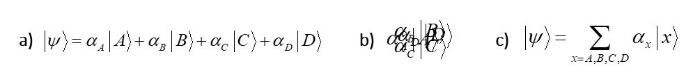
You might be wondering how the model being described here relates to the canonical, vector-based formalism of quantum theory (QT), i.e., based on Hilbert space and the Schrodinger equation. Each of the state-representing sets, ψ(A)-ψ(D), are the basis functions. And, the binary weight matrix, together with the simple algorithm described above, is the operator. But here’s the crucial difference. The basis functions of QT are formally vectors and thus have the semantics of 0-dimensional points. This zero dimensionality, i.e., zero extension, of the represented entity is what allows the formalism to represent a basis state by a single (localized) symbol, i.e., using a localist representation. Fig. 9a shows this for the 4-state system we’ve been using: the four basis functions each has its own dedicated symbol and the four symbols are formally disjoint. But they are not merely formally disjoint: they are physically disjoint in any physical reification of the formalism in which operations are performed. We do not write all these symbols down on top of each other, i.e., superpose them, as in Fig. 9b. That becomes a blur and meaningless, and cannot be operated on by the formal mechanics of QT. Yes, we can abbreviate the fully expanded sum with a single symbol, i.e. the summation symbol (with the relevant indexes), as in Fig. 9c. But again, actual computations, i.e., applications of the Schrodinger equation to update the system, are formally outer products of the fully expanded summations, i.e., requiring 2Nx2N multiplications, where N is the number of basis functions.
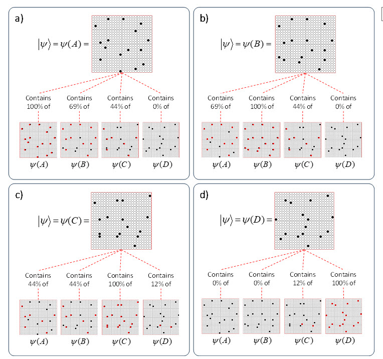
Comparing Fig. 10 to Fig. 9 shows the stark representational difference between my theory and QT. Fig. 10a shows the formal symbol, ψ(A), representing state A: it’s the set of Q=16 active (black) bits in the fermionic field. And below it we show the strengths of presence of each of the four basis states in state A (repeated from Fig. 2a). Thus these basis states are not orthogonal as are the basis states in QT’s Hilbert space representation. Again, the physical reification of each individual basis state, i.e., ψ(X), simultaneously is both: i) the state X at full strength because all Q of ψ(X)’s bits are active; and ii) all the other basis states, with strengths proportional to their intersections with ψ(x). Thus, unlike the situation for QT (i.e., Fig. 9b), when you look at any one of the four set-based representations in Fig. 10 you are looking at the physical superposition of all the system’s states, just with different degrees of strength for the different states depending on which state is fully active. This is superposition realized in a purely classical way, as set intersection. There is no blurriness and the active sparse set is directly operated on by the mechanics of the formalism. And, crucially, that operation consists of a number of atomic operations that depends on the number of physical representational units (the number of bits comprising F), not on the number of represented basis states. Also, unlike the formalism of QT, the representation of the basis states per se and of the probabilities of the states (which in QT are formally probability amplitudes, but in my theory, are formally likelihoods) per se are formally co-mingled: all of the information about the state is distributed out homogeneously throughout all Q of its bits.
The stark difference described above all comes down to the fact that in QT, states are represented by vectors but in my theory, they are represented by sets. A vector is formally equivalent to a point in the vector space. A point is a 0-dimensional object, i.e., it has no extension. But a set fundamentally does have extension. This is because the elements of a set are unordered (whereas those of a vector are ordered). This means that from an operational standpoint, there is no shorter representation of a set than to explicitly “list”, i.e., explicitly activate, all its elements. While we can assign a single symbol, e.g., “ψ(A)”, as the name of a set, the formal representation of any operation on a set must include symbols representing every element in the set. Thus, to specify the outcome of the application of the state update operator at time t+1, we must show you the full matrix of weights, i.e., the state of every weight, or at least the state of every weight leading from every active element at t, as in Fig. 8. The unorderedness of sets has crucial implications regarding the physical realizations of the formal objects and of the operations on the formal objects. This relates directly to Jacob Barandes’s “category problem” of QT, which concerns the relation between “happening” and “measuring”. See his talk.
..Next Section coming soon…
I’ll continue to explain and elaborate on how the functionality of superposition is fully achieved by classical set intersection. In particular, “fully achieving the functionality” includes achieving the computational efficiency (i.e., exponential speed-up) of quantum superposition.
And, I’ll fully explain the completely classical explanation of entanglement that comes with this theory based on representing states by sparse sets. An essay of mine from 2023 already explains entanglement in my formalism, but it needs updating.
I’ll elaborate on how this core theory generalizes to explain how the three large-scale spatial dimensions of the universe are emergent. This has already been explained at length in an earlier essay (2021), but that also needs significant updating.
I’m continuing to learn a lot about some other quantum foundation theories, i.e., Barandes’ “Indivisible Stochastic Processes”, Finster’s “Causal Fermions”, and “Causal Sets”, and will be elaborating on the relationships that exist between those theories and mine. But, it is immediately clear from their lectures that at least the latter two are vector-based theories (despite their names). And it is true that none of these three theories has yet proposed a physical underpinning of the probabilities, as I have.
References
- Rinkus, G., A Combinatorial Neural Network Exhibiting Episodic and Semantic Memory Properties for Spatio-Temporal Patterns, in Cognitive & Neural Systems. 1996, Boston U.: Boston.
- Rinkus, G., A cortical sparse distributed coding model linking mini- and macrocolumn-scale functionality. Frontiers in Neuroanatomy, 2010. 4.
- Rinkus, G. A Radically New Theory of How the Brain Represents and Computes with Probabilities. in Machine Learning, Optimization, and Data Science. 2024. Champlinaud: Springer Nature Switzerland.
- Rinkus, G.J., Sparsey™: event recognition via deep hierarchical sparse distributed codes. Frontiers in Computational Neuroscience, 2014. 8(160)